
📚 GPU Acceleration
This document reviews the main themes and key takeaways from Deep Learning Systems: Algorithms and Implementation** at Carnegie Mellon University, taught by J. Zico Kolter and Tianqi Chen.
This lecture summarizes key concepts and techniques related to GPU (Graphics Processing Unit) acceleration, particularly within the context of deep learning and linear algebra operations. The information is drawn from two primary sources: a lecture transcript (“Lecture - 12 GPU Acceleration”) and a corresponding slide deck (“https://dlsyscourse.org/slides/12-gpu-acceleration.pdf”).
I. Core Concepts: GPU Architecture & Programming Model
CPU vs. GPU Architecture
- CPU (Central Processing Unit): Designed for flexibility with a strong “commander unit” (control unit) capable of handling diverse tasks, including branching, context switching. Emphasizes flexible control.
- GPU (Graphics Processing Unit): Employs a large number of “soldiers” (compute cores) under the control of fewer “commanders” (control units). Optimized for highly parallel, arithmetic-intensive tasks, where the same operation is performed on large datasets.
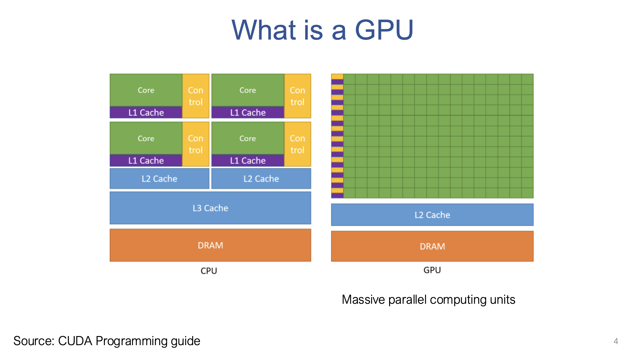
“A typical CPU will have a very strong Commander unit…that allows us to do different kind of tasks…On other hand…we are doing a lot of similar things…you want a huge amount of soldier that go ahead and perform a task…” 💡
Massive Parallelism
GPUs provide significant speedups in specific tasks compared to CPUs, often in the range of 10x to 100x.
“By leveraging your GPU you can usually observe more than 10 X or sometimes 100 X speedup versus traditional computing…GPU itself is kind of indispensable nowadays in order to run deep learning works” 🚀
SIMT (Single Instruction, Multiple Threads) Programming Model
GPU programming employs SIMT, where all threads execute the same code (kernel) but on different data.
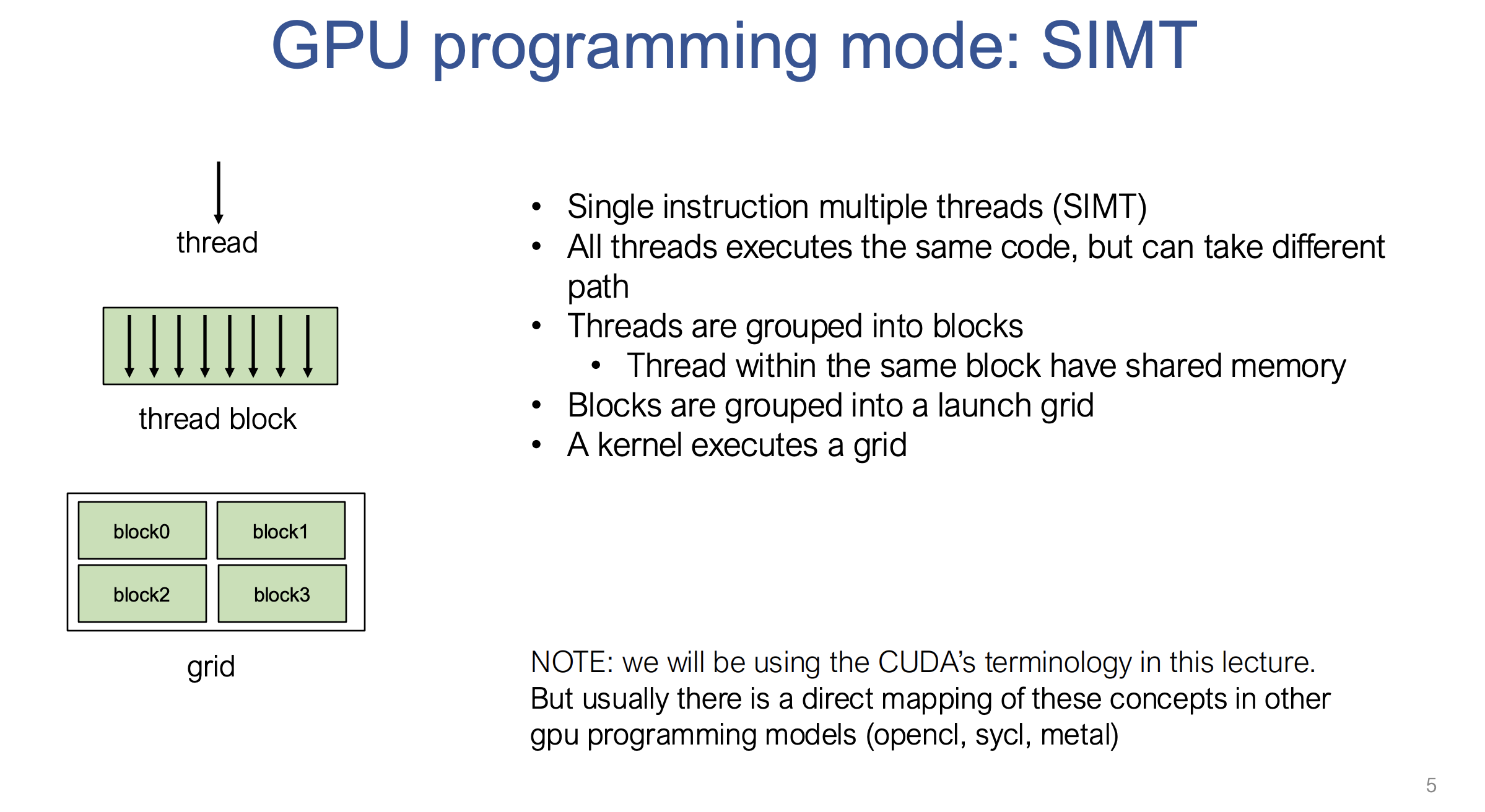
“All threads executes the same code, but can take different path” 🔄
How to read the SIMT figure
SIMT is best read as “many independently addressed threads begin by following the same kernel instructions.” A warp is the hardware scheduling unit on NVIDIA GPUs and normally contains 32 threads. The threads have different thread IDs, so an elementwise assignment acts on a different element in every thread. They may take different branches, but a branch that splits a warp can cause the paths to be executed serially under masks. This is why uniform control flow is usually preferable.
Threads, Thread Blocks, and Grids
- Threads: Individual execution units that perform computations.
- Thread Blocks: Threads are grouped into blocks, which share common resources such as shared memory.
- Grid: Thread blocks are further grouped into a launching grid when a GPU kernel is executed.
“we’re going to group the thread onto what we call blocks and the threads within the same blocks also share uh some kind of common resources…finally all the blocks are then grouped into what we call a launching grid…” 🎯
Context
Each thread has its own context, especially its unique locations (thread ID and block ID), allowing for varied data access and storage even though the same code is executed.
From local IDs to a global element
For a one-dimensional launch, the usual mapping is:
global index = blockDim.x × blockIdx.x + threadIdx.x
With four threads per block, block 0 owns global indices 0 through 3 and block 1 owns 4 through 7:
block 0: threadIdx.x = 0, 1, 2, 3  ->  i = 0, 1, 2, 3
block 1: threadIdx.x = 0, 1, 2, 3  ->  i = 4, 5, 6, 7
The same kernel code runs for every row above. The ID calculation is what gives each invocation a different data element. A block is also the boundary for shared memory and for the block-wide synchronization primitive used later.
CUDA (Compute Unified Device Architecture)
NVIDIA’s programming model for GPUs, the primary focus of the lecture, but similar models exist (OpenCL, SYCL, Metal).
Data Parallelism
The ability to execute tasks on each data element independently is crucial for efficient GPU utilization.
“The ability to parallelize depends on how much independence we have across each element of computation…” 🔢
Operations with data dependencies require more complex parallel implementations such as parallel scan, instead of simple data parallelism.
II. GPU Programming Example: Vector Addition
CPU Implementation
A simple for loop iterates over the array elements to perform the addition.
GPU (CUDA) Implementation
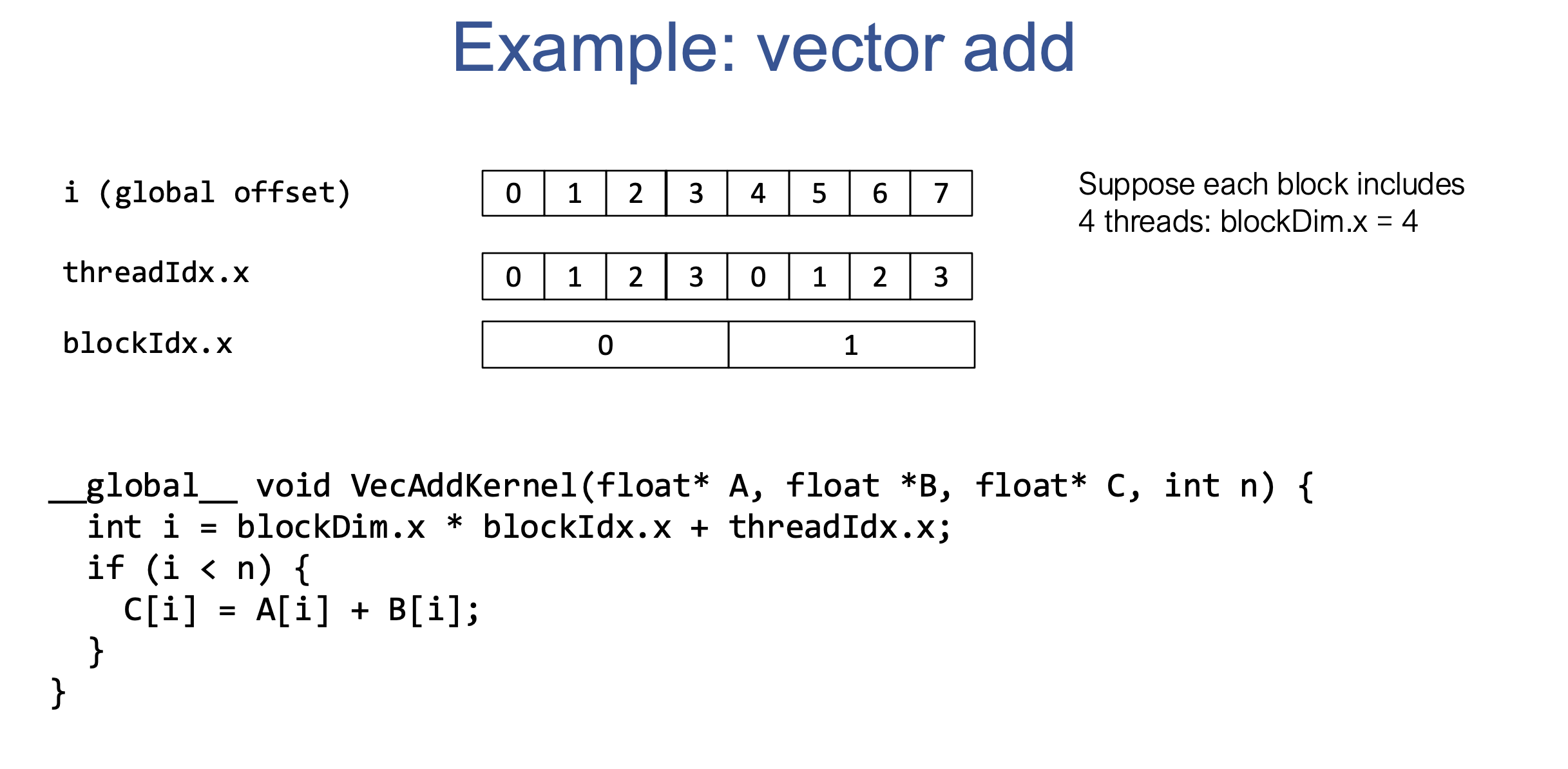
- A kernel function (
__global__ void VecAddKernel(...)) executes on the GPU. - Each thread calculates a global index based on its block and thread ID (
int i = blockDim.x * blockIdx.x + threadIdx.x;). - Threads perform additions on specific array elements concurrently.
“Each of Str it’s only doing one computation right…load from A, load from B, do the addition, and then write result back on C…” 🧮
Line-by-line: the device kernel
The figure contains the complete one-dimensional vector-add kernel:
__global__ void VecAddKernel(float* A, float* B, float* C, int n) {
  int i = blockDim.x * blockIdx.x + threadIdx.x;
  if (i < n) {
    C[i] = A[i] + B[i];
  }
}
- The global qualifier means host code can launch this function and its body runs on the device.
- A, B, and C are device pointers; indexing them accesses GPU global memory.
- The index expression converts a thread’s position inside its block into an array index across the whole grid.
- The guard is required because launches are normally rounded up to a convenient block size. For example, n = 1,000 and 256 threads per block needs four blocks (1,024 threads); the final 24 threads must do nothing.
- Every active thread performs exactly two global loads, one add, and one global store. There is no communication between threads, so vector add is an ideal data-parallel operation.
Because consecutive threads produce consecutive i values, a warp normally loads A[i] and B[i] from adjacent global-memory addresses. For 32-bit floats, lanes 0 through 31 access 128 consecutive bytes. The GPU can combine that warp-level request into a small number of efficient memory transactions; this is coalesced access. A strided mapping such as each lane reading A[lane × 32] scatters the same warp across a much wider range and usually needs more transactions.
Host-Side Code
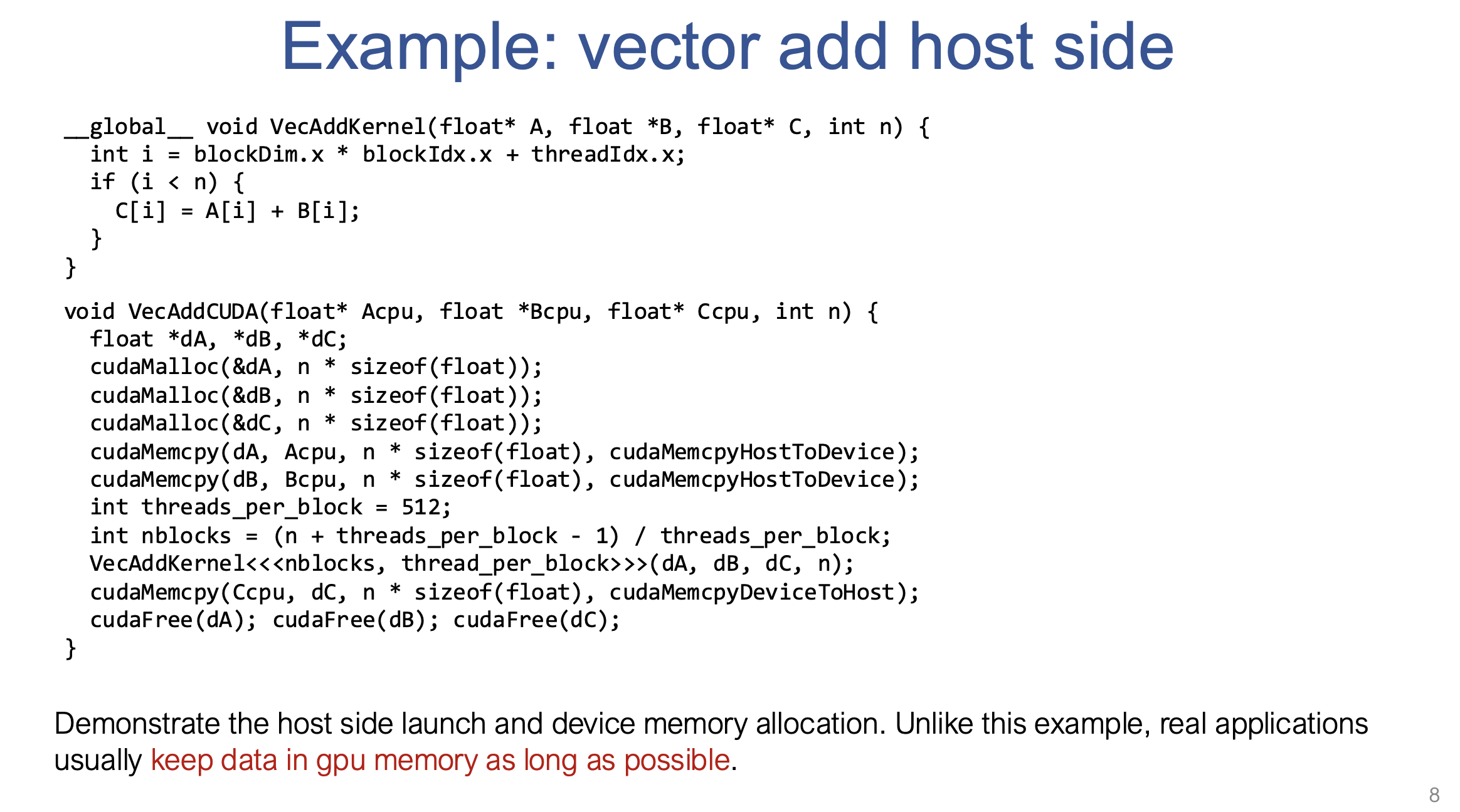
- Allocates memory on the GPU using
cudaMalloc. - Copies data from CPU (host) memory to GPU (device) memory using
cudaMemcpy. - Launches the kernel with specified numbers of threads and blocks.
- Copies results back to the CPU using
cudaMemcpy. - Frees allocated GPU memory using
cudaFree.
“when you call CA memory copy these operations help us to be able to take uh original memory and copy the data onto the corresponding regions on GPU…we’re going to launch a CUDA kernel with you know so many threads per block and number of blocks by passing in the GPU pointer” 🎯
Line-by-line: host allocation, launch, and return
The host code uses dA, dB, and dC for device pointers, distinct from the CPU pointers Acpu, Bcpu, and Ccpu:
cudaMalloc:  reserve three device buffers
cudaMemcpy:  copy A and B from host memory to device memory
<<<grid, block>>>: launch one kernel invocation per GPU thread
cudaMemcpy:  copy C from device memory back to host memory
cudaFree:    release the three device buffers
The grid-size expression (n + threads_per_block - 1) / threads_per_block is integer ceiling division. With n = 1,000 and 512 threads per block, it produces 2 blocks, which launches 1,024 threads; the kernel’s bounds guard handles the extra threads. In production code, every CUDA API call and kernel launch should also be checked for errors, and copies should be avoided between dependent GPU operations whenever possible.
Key Point
Real-world GPU applications minimize CPU-GPU data transfers, instead aiming to keep data in GPU memory as long as possible to reduce bottlenecks.
“Real world applications really try to keep data in GPU memory as long as possible” 🏃♂️
III. GPU Memory Hierarchy
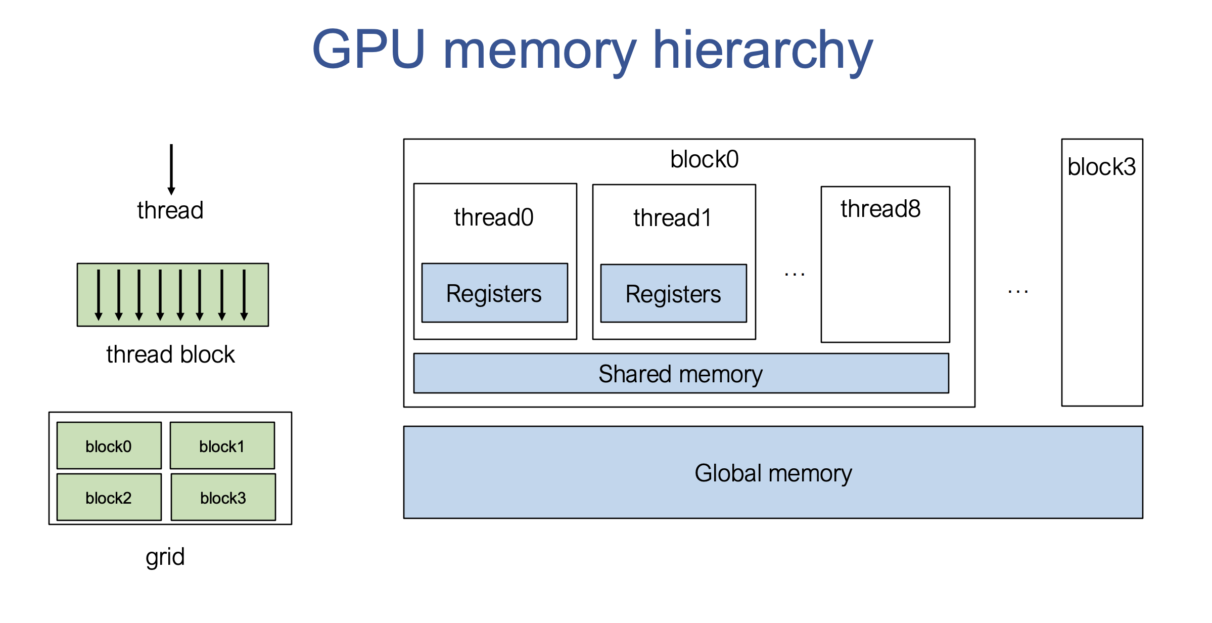
Two-Level Hierarchy
- Global Memory: Main memory of the GPU, allocated via functions like
cudaMalloc. Slower, shared across the entire GPU. - Shared Memory: Fast, on-chip memory shared by threads within the same block. Used for data reuse and optimization.
- Registers: Local memory for each thread.
- Stream Multiprocessors (SM): Blocks are mapped to SMs, which contain multiple computing cores. Shared memory is associated with each SM.
Scope is the important part
The same word “shared” can be misleading without scope:
global memory:  visible to every block; large, high-latency device DRAM
shared memory:  visible only to threads in one block; explicit on-chip scratchpad
registers:      private to one thread; fastest and smallest
Two blocks cannot directly share their shared-memory array, even when both happen to execute on the same SM. A thread may also use more register variables than fit in physical registers; the compiler can spill those values to slower local memory. Therefore “put everything in registers/shared memory” is not a free optimization.
IV. Optimization: Shared Memory & Window Sum
The window sum example demonstrates how shared memory can be used to optimize memory access and improve the performance of GPU computations. The goal is to compute the sum of elements within a sliding window. 🌐
Important convention: the exact code figure below uses a forward window. With RADIUS = 2, B[i] sums A[i] through A[i + 4]. A centered radius-2 convention would instead sum A[i - 2] through A[i + 2]. Both use five values, but they need different boundary handling; the worked code follows the forward-window form.
Imagine an input array A with n elements and a window width of 5. For each output element B[i], the figure calculates the sum of the five consecutive values A[i] through A[i + 4].
For simplicity, assume:
- RADIUS is 2, so the code needs two additional halo values after the four output positions owned by a block.
- We have 4 threads per block.
1. Naive Approach 🛠️
In the naive implementation, each thread would independently load the required data from global memory and compute the sum for its corresponding output element.
- Problem: Threads load overlapping data. For example, Thread 0 will load the elements
A[0], A[1], A[2], A[3], A[4], while Thread 1 will loadA[1], A[2], A[3], A[4], A[5]. This leads to redundant memory accesses and unnecessary overhead.
2. Optimized Approach Using Shared Memory 🔥
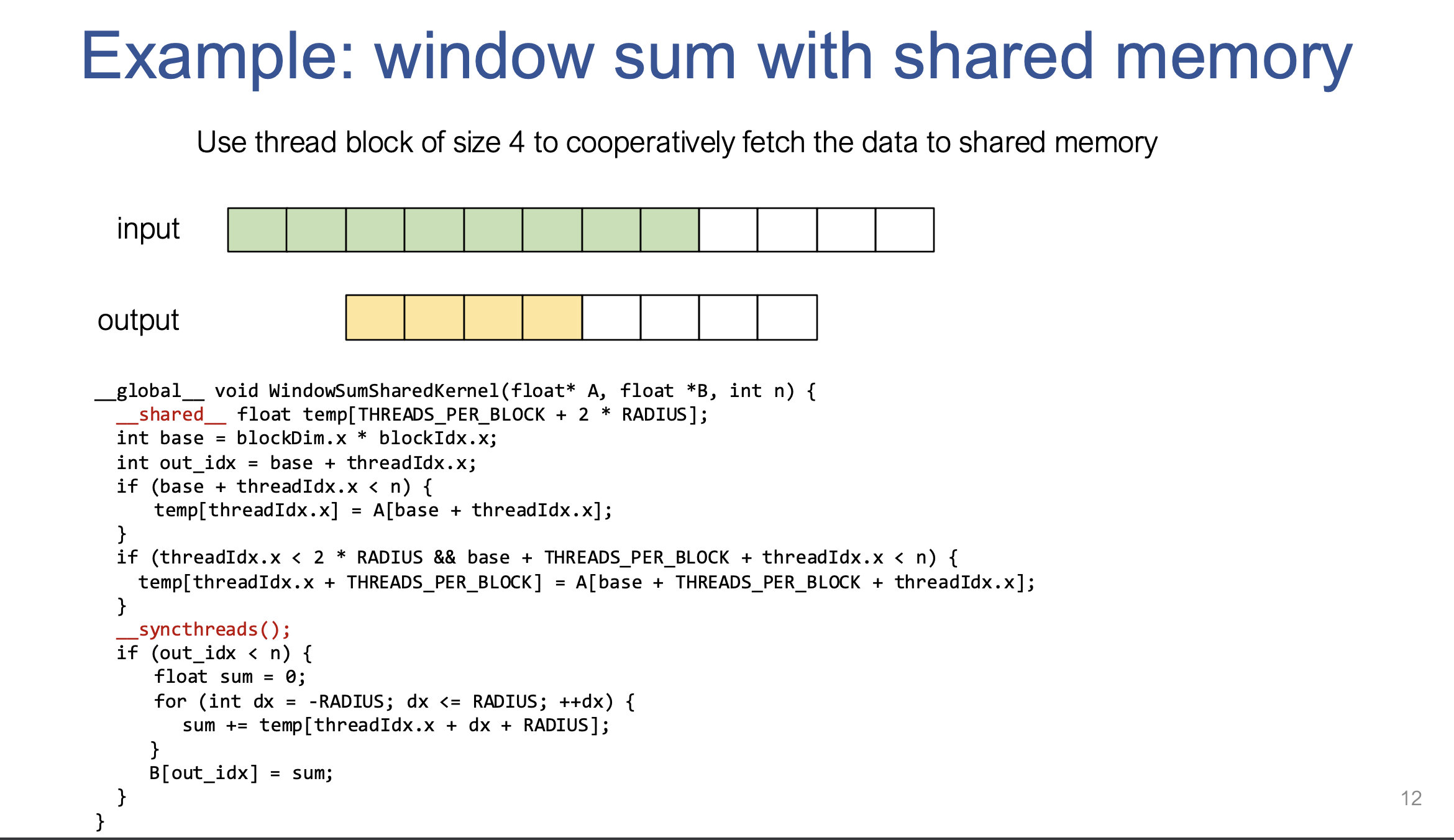
In the optimized version, we use shared memory to load the data once per block, and then allow all threads to access it. This minimizes redundant global memory accesses and improves performance.
How to read the code in the figure
The figure uses THREADS_PER_BLOCK = 4 and RADIUS = 2. For block 0:
base = 4 × blockIdx.x = 0
thread 0, 1, 2, 3 first load A[0], A[1], A[2], A[3] into temp[0..3]
the first 2 × RADIUS = 4 threads also load A[4], A[5], A[6], A[7] into temp[4..7]
After this cooperative fetch, the shared array is one contiguous input window:
temp = [A0, A1, A2, A3, A4, A5, A6, A7]

thread 0 sums temp[0..4] -> B0 = A0 + A1 + A2 + A3 + A4
thread 1 sums temp[1..5] -> B1 = A1 + A2 + A3 + A4 + A5
thread 2 sums temp[2..6] -> B2 = A2 + A3 + A4 + A5 + A6
thread 3 sums temp[3..7] -> B3 = A3 + A4 + A5 + A6 + A7
The block-wide synchronization call is essential: without it, one thread could begin reading temp[4] before the thread responsible for loading A4 has written it. The barrier synchronizes only the current block, which is exactly the set of threads sharing this temp array.
The slide omits a full boundary policy. Near the end of the input, a production implementation might launch only n - 2 × RADIUS valid outputs, add zero padding, clamp indices, or use a separate boundary kernel. Loading guards alone do not define what a five-element window should mean when fewer than five input values remain.
Key Steps:
-
Shared Memory Allocation: Each block of threads has access to a section of shared memory. We allocate enough space in shared memory to hold all the elements required by the threads in the block. For a radius of
2and4threads per block, we need a total of4 threads + 2 * radius = 4 + 4 = 8 elementsin shared memory. - Loading Data into Shared Memory:
- Each thread loads its corresponding element into shared memory.
- To ensure all threads can access data from neighboring threads (to cover the full window), threads at the beginning of the block will also load data beyond their own index.
-
Synchronizing Threads: The function
__syncthreads()ensures that all threads have finished loading their data into shared memory before any of them begin computing the sum. - Computing the Sum: After loading the data, each thread calculates the sum of elements within its sliding window using the data from shared memory. Since all threads have access to the same shared memory, they can work together without redundant memory accesses.
Example with 4 Threads:
Let’s say the array A = [1, 2, 3, 4, 5, 6, 7, 8, 9] and we have 4 threads per block with a radius of 2.
-
The shared memory will hold the data
A[0], A[1], A[2], A[3], A[4], A[5], A[6], A[7]. This way, each thread can access its own element and also the elements required by its neighboring threads. - Thread 0 calculates the sum of
A[0] + A[1] + A[2] + A[3] + A[4]. - Thread 1 calculates the sum of
A[1] + A[2] + A[3] + A[4] + A[5]. - Thread 2 calculates the sum of
A[2] + A[3] + A[4] + A[5] + A[6]. - Thread 3 calculates the sum of
A[3] + A[4] + A[5] + A[6] + A[7].
Benefits:
- Memory Efficiency: Each thread only loads the data it needs into shared memory once, instead of repeatedly loading the same data from global memory.
- Faster Access: Shared memory is much faster to access than global memory, leading to a significant speedup in computation.
- Cooperation Between Threads: Threads within a block cooperate to load the data into shared memory, making the computation more efficient.
3. How It Works in Shared Memory
In the GPU architecture:
- Global Memory: Is slower and shared across all threads of all blocks.
- Shared Memory: Is much faster but only accessible by threads within the same block. It’s ideal for situations where threads need to perform similar operations on neighboring elements of large datasets.
Final Thoughts:
- By using shared memory, we avoid the overhead of redundant global memory accesses, and the threads in a block work together more efficiently.
- This approach is especially helpful for tasks like convolution operations, matrix multiplications, and other tasks where threads need to perform similar operations on neighboring elements of large datasets.
This process greatly speeds up computations, particularly in deep learning or scientific computing tasks that require processing large arrays of data. 🎯
4. Step-by-Step Code Explanation 🔍
- Shared Memory Allocation: The shared memory array
tempholds data for the entire block of threads. It’s sized based on the number of threads per block and the radius of the window. 🏗️ - Index Calculations: The
basevariable calculates the starting index for the block, andout_idxis the output index for the current thread. ⏱️ - Loading Data into Shared Memory: Each thread loads its corresponding element from global memory into shared memory (
temp). 🌍 - Handling Edge Elements: Threads at the beginning of the block also load additional data into shared memory to ensure the entire window is covered. 🛠️
- Synchronization: This ensures all threads have finished loading data into shared memory before moving forward. 🔒
- Sum Calculation: Each thread sums the values within the sliding window using data from shared memory. 🧮
5. Advantages of Shared Memory 🚀
- Reduced Global Memory Access: Shared memory significantly reduces the number of accesses to global memory. Threads load only a minimal number of elements. 🚫
- Increased Memory Reuse: Data in shared memory can be reused by all threads in the block, eliminating redundant loads. 🔁
- Faster Memory Access: Shared memory is much faster to access than global memory, leading to performance improvements. ⚡
V. Case Study: Matrix Multiplication on GPU
Tiling
Dividing large problems into smaller subproblems (tiles) to improve data locality and reuse.
Register Tiling
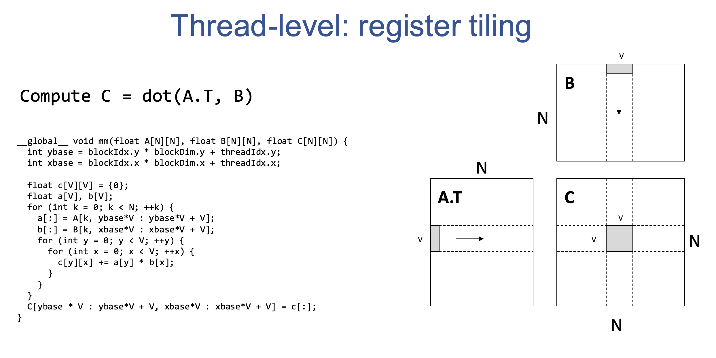
- Each thread computes on a submatrix (V x V) of the output matrix.
- Input data (A and B) is loaded into registers for fast access.
- Increases data reuse within a single thread.
How to read the register-tiling figure
The figure uses the convention C = dot(A transpose, B). A thread first computes its two-dimensional location:
ybase = blockIdx.y × blockDim.y + threadIdx.y
xbase = blockIdx.x × blockDim.x + threadIdx.x
The thread does not own one scalar output. It owns a V × V square whose top-left corner is (ybase × V, xbase × V). For V = 2, a thread with ybase = 1 and xbase = 2 owns:
C rows 2 and 3, columns 4 and 5

c = [[C[2,4], C[2,5]],
     [C[3,4], C[3,5]]]
For one reduction index k, that thread loads two values from the selected row of A and two from the selected row of B into its registers:
a = [A[k,2], A[k,3]]
b = [B[k,4], B[k,5]]
It then performs the small outer-product update:
c[0,0] += a[0] × b[0]       c[0,1] += a[0] × b[1]
c[1,0] += a[1] × b[0]       c[1,1] += a[1] × b[1]
The loop over k repeats this update. The four c values remain in registers for the entire reduction and are written to global memory only once. That is why one A value is reused for V output columns and one B value is reused for V output rows inside the same thread.
Shared Memory Tiling
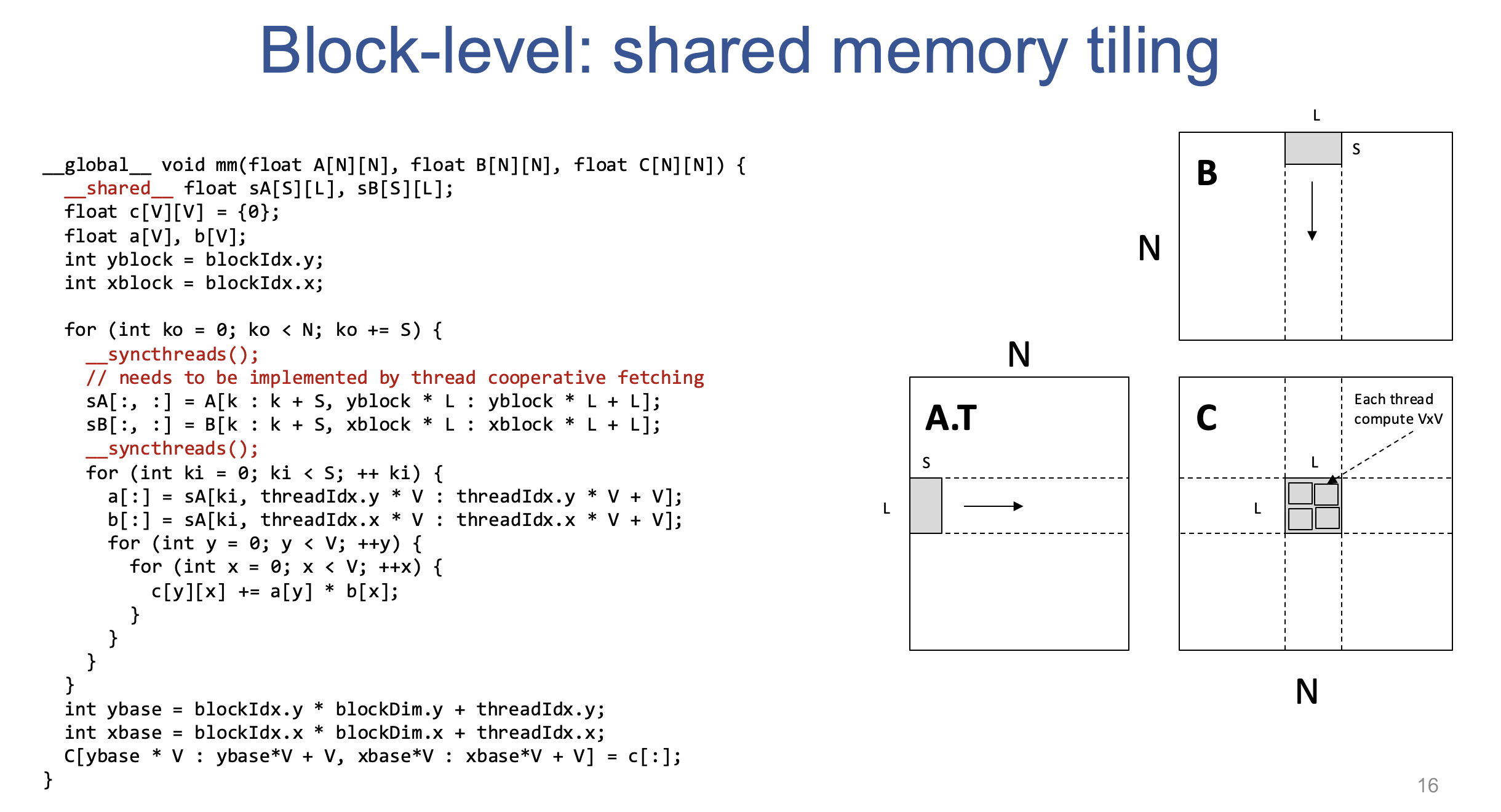
- Each block computes a submatrix (L x L), and each thread computes a submatrix of V x V.
- Input blocks of A and B are first loaded into shared memory for reuse across all threads in the block.
- Threads load from the shared memory into registers to perform computations.
“We are going to first iterate over the reduction dimension in each case we want to be able to fetch the corresponding data first onto the shared memory” 🔄
How to read the shared-memory-tiling figure
The block-level figure adds a cooperative layer above the register tile:
L = width/height of the output tile owned by one block
V = width/height of the smaller output tile owned by one thread
S = width of one reduction-dimension chunk
For one K chunk, the block needs two panels:
sA[S][L]: S rows from A, spanning the block's L output rows
sB[S][L]: S rows from B, spanning the block's L output columns
All threads cooperate to copy these panels from global memory into shared memory. Only after every required element is present may the threads read the panels and update their private register tiles. Conceptually each K chunk has two barriers:
- a barrier after the cooperative loads, before anyone consumes the shared arrays;
- a barrier before the next chunk overwrites the arrays, after everyone has finished consuming them.
The slide shows a synchronization at the top of the next loop iteration, which serves as the second barrier for the previous iteration.
A small concrete configuration
Take L = 16, V = 4, and S = 8:
one block computes a 16 × 16 output tile of C
the block contains (16 / 4) × (16 / 4) = 4 × 4 = 16 threads
each thread owns one 4 × 4 register tile of C
each K phase cooperatively loads an 8 × 16 panel from A and an 8 × 16 panel from B
The two shared panels hold 256 floats total. The 16 threads divide those loads among themselves, then each thread repeatedly reads its needed row fragments into a and b registers and updates its 16 c accumulators. In this configuration:
- an element fetched from global memory to shared memory can help many threads in the block;
- an element fetched from shared memory to registers can help multiple multiply-adds in the one thread’s 4 × 4 output tile;
- completed c values are stored to global memory after all S-wide K phases are accumulated.
One detail in the slide pseudocode is worth calling out: the line that loads the b register vector is displayed as reading sA. Its intended source is sB, otherwise both vectors would come from A and the multiplication would be incorrect.
Thread-level and block-level tiling: a small worked example
The terms become clearer with a matrix small enough to calculate by hand. Use ordinary row-major multiplication C = A × B:
A =                         B =

[a00 a01 | a02 a03]         [b00 b01]
[a10 a11 | a12 a13]         [b10 b11]
                            ---------
                            [b20 b21]
                            [b30 b31]
A is 2 × 4, B is 4 × 2, and C is 2 × 2. The vertical/horizontal separators split the K dimension into two tiles: K = 0,1 and K = 2,3. For example:
c00 = a00×b00 + a01×b10 | + a02×b20 + a03×b30
c01 = a00×b01 + a01×b11 | + a02×b21 + a03×b31
c10 = a10×b00 + a11×b10 | + a12×b20 + a13×b30
c11 = a10×b01 + a11×b11 | + a12×b21 + a13×b31
Block-level tiling: threads share an input tile
Imagine a 2 × 2 block of threads:
T00  T01          T00 owns c00; T01 owns c01
T10  T11          T10 owns c10; T11 owns c11
For the first K tile, the threads cooperatively load:
shared A =                 shared B =

[a00 a01]                  [b00 b01]
[a10 a11]                  [b10 b11]
One simple assignment is T00 loads a00/b00, T01 loads a01/b01, T10 loads a10/b10, and T11 loads a11/b11. The block then executes __syncthreads(). Only after every writer has finished may T00 compute a00×b00 + a01×b10, T01 compute a00×b01 + a01×b11, and so on. The block repeats the sequence with the second K tile:
shared A =                 shared B =

[a02 a03]                  [b20 b21]
[a12 a13]                  [b30 b31]
The important reuse is across threads: a00 contributes to both c00 and c01, and b00 contributes to both c00 and c10. Shared memory lets the block load each value once from global memory, then reuse it for those outputs.
Thread-level tiling: one thread owns several output values
Instead, one thread can own the whole 2 × 2 output tile:
one thread owns [c00 c01]
                  [c10 c11]
At K = 0 it privately loads a00/a10 and b00/b01, then performs the small outer-product update:
c00 += a00×b00       c01 += a00×b01
c10 += a10×b00       c11 += a10×b01
The thread repeats this for K = 1, 2, and 3. Its four accumulators and its temporary A/B fragments are private state, normally held in registers. No barrier is required because no other thread reads or writes them. The reuse is inside one thread: a00 is reused for c00/c01, and b00 for c00/c10.
Combined tiling: the usual high-performance design
Real kernels normally combine the two levels. A block owns a larger L × L tile of C and cooperatively loads A/B panels into shared memory. Each thread then reads its portion of those panels and accumulates a smaller V × V C tile in registers:
global memory → shared-memory tile reused across a block
              → register tile reused within one thread
              → final C values in global memory
For L = 16 and V = 2, an 8 × 8 block of 64 threads produces one 16 × 16 C tile; every thread owns four C values. This is the same two-level structure shown in the shared-memory tiling figure above.
What synchronization does—and does not—do
__syncthreads() is a barrier for the current block only. It has two jobs in each K phase: first, make cooperative shared-memory loads visible before reads; second, ensure every reader is finished before the next phase overwrites the shared arrays. It does not merge partial results, add values automatically, or synchronize separate blocks. Each thread explicitly updates its own C accumulators and writes its own output locations. A host-side copy or an explicit cudaDeviceSynchronize() waits for the whole preceding kernel when the CPU needs the finished result.
Cooperative Fetching
Individual threads cooperatively fetch data from global memory into shared memory in an efficient way.
“Each of the threads in here is going to correspond to a cooperative fetching among multiple threads where each of the threads is going to perform one part of the job” 🔗
Memory Reuse Analysis
- Global memory to shared memory reuse.
- Shared memory to register reuse.
Careful selection of tiling factors (L and V) is crucial for performance and is often done through auto-tuning.
Trade-offs
Choosing the correct values of L and V is difficult due to multiple factors, including:
- Number of registers available for each thread vs total number of threads in a single Stream Multiprocessor (SM).
- Size of shared memory that affects how many thread blocks can fit into each SM.
- Data loading speed due to memory access patterns.
“When we are trying to pick for example the values of L and V, it is something that is affected by a lot of factors” 🧠
Details
🚀 GPU Matrix Multiplication: Register and Shared Memory Tiling
Matrix multiplication on GPUs can be significantly accelerated using techniques like register tiling and shared memory tiling. These methods optimize memory access and data reuse, crucial for maximizing performance on GPUs. Let’s break it down step by step! 🔧
1. The Goal: Matrix Multiplication 🎯
-
We want to compute matrix multiplication:
C = A * B
More specifically:
Cᵢⱼ = Σₖ Aᵢₖ * Bₖⱼ
This can also be written as:
C = dot(Aᵀ, B), meaning:
Cᵢⱼ = Σₖ Aₖᵢ * Bₖⱼ -
The goal is to perform these calculations in parallel on the GPU for speedup.
2. Register Tiling (Thread-Level Tiling) 🧱
📌 Concept:
- Register tiling divides matrices into smaller submatrices that fit into the GPU’s registers.
🔧 Mechanism:
- Submatrix of size V x V (where V is the tiling factor) is allocated per thread.
- Each thread computes one V x V submatrix of the output matrix C.
- Two temporary arrays, a and b, of size V are created in each thread’s registers.
- Strips of data from matrices A and B are loaded into a and b.
- The dot product is computed, and results accumulate in the register array c.
- Finally, the computed submatrix is written back to global memory.
🚀 Advantages:
- Memory Reuse: Each element of A and B is reused V times within the registers.
- Speed: Register access is very fast, boosting performance.
3. Shared Memory Tiling (Block-Level Tiling) 🧩
📌 Concept:
- This technique leverages shared memory for further optimization, enabling threads in a block to share data.
🔧 Mechanism:
- Each thread block computes a L x L submatrix of C (L = tiling factor).
- Each thread performs a V x V computation inside this block.
- Shared memory arrays, sA and sB, of size S x L are allocated.
- Threads cooperate to load data from global memory into shared memory.
- After loading, threads access data from shared memory into registers (a and b) for computation.
- Results are stored in the register array (c) and written back to global memory.
🚀 Advantages:
- Increased Reuse: Data loaded into shared memory is reused across threads.
- Cooperative Loading: Threads load data together, reducing redundant loads.
- Higher Performance: Combining register tiling with shared memory tiling maximizes efficiency.
4. Memory Reuse Analysis 📊
- Global → Shared Memory: Data reuse factor of L. Memory loads reduced by L times.
- Shared → Registers: Data reuse factor of V. Memory loads reduced by V times.
🔹 Total Reduction:
- Global to Shared:
2 * N³ / L - Shared to Registers:
2 * N³ / V
5. Cooperative Fetching 🤝
- Threads work together to load data into shared memory, avoiding redundancy.
🔧 How It Works:
- nthreads = blockDim.y * blockDim.x (total threads in a block).
- Each thread has a unique ID:
tid = threadIdx.y * blockDim.x + threadIdx.x - A loop (j) distributes the load:
Threads calculate the coordinates:
y = (j * nthreads + tid) / L
x = (j * nthreads + tid) % L - Data is loaded as:
s[y, x] = A[k + y, yblock * L + x]
6. Choosing L and V ⚖️
Choosing the best values for L and V involves balancing several factors:
- Register Usage:
- Larger V → More reuse within threads but fewer concurrent threads.
- Shared Memory Size:
- Larger L → More reuse but limits blocks per Streaming Multiprocessor (SM).
- Thread Parallelism:
- More threads → Better performance (hides latency).
🔹 Trade-off:
- Fewer threads with large registers OR
- More threads with smaller registers.
🔹 Auto-Tuning:
- Test various L and V values to find the optimal combination.
VI. Further GPU Optimization Techniques
- Continuous Memory Access: Ensuring threads read from contiguous regions of memory to optimize memory access.
- Shared Memory Bank Conflict: Avoid conflicts when multiple threads in a warp (subgroup of threads) access the same memory banks.
- Software Pipelining: Overlapping data loading with computation for increased throughput.
- Warp Level Optimizations: Exploiting the smaller granularity of warps for collective computations.
- Tensor Cores: Using specialized hardware units on modern GPUs for accelerated matrix operations.
Reading these techniques through the examples
- Continuous (coalesced) access: The vector-add figure is already the good case: neighbouring lanes access neighbouring floats. In a matrix kernel, make the lane-varying index follow the contiguous dimension of the actual memory layout.
- Shared-memory bank conflicts: Shared memory is divided into banks so several threads can often read different addresses at once. A bad access pattern maps many distinct addresses to the same bank, serializing the accesses. Padding a two-dimensional shared array by one column is a common way to change the mapping.
- Software pipelining: The shared-matmul figure has a load phase and a compute phase for every K tile. A more advanced kernel starts loading tile K + 1 while it computes tile K, so global-memory latency is hidden behind useful arithmetic.
- Warp-level primitives: A reduction within one warp can use shuffle instructions to exchange register values without first writing them to shared memory. This is faster but only works within that 32-thread warp scope.
- Tensor Cores: These specialized units multiply small matrix fragments extremely quickly. They still need the same surrounding work: sensible layouts, tiled loads, accumulation, and enough parallel blocks to keep the GPU busy.
“All those techniques are important to really get us the maximum benefit of a GPU accelerator” 🎯