nano-vLLM Part 2: Block Tables, KV Cache, and the Path to the GPU

nano-vLLM Part 2: Block Tables, KV Cache, and the Path to the GPU

Part 1 followed a request through waiting, running, prefill, decode, and preemption. This post goes below the scheduler’s decision. Once it says, “sequence A may run,” how does the program know where A’s keys and values live on the GPU? How can two requests reuse the same prefix? And what exactly is prepared before ModelRunner.run() calls the model?

The answer spans two layers of the system:

CPU control plane
  Scheduler + BlockManager assign stable logical block IDs to each Sequence
        ↓
GPU data plane
  ModelRunner turns those IDs into tensors; attention kernels use them to
  read and write the global per-layer KV cache

The main source files are block_manager.py, model_runner.py, and attention.py. I use a toy block size of four tokens in the examples. nano-vLLM’s configured default is 256; the mechanics are identical.

1. The three things that are easy to conflate

Before tracing an example, separate these three objects.

Object	Lives where	Who owns it	What it means
seq.block_table	CPU Python object	BlockManager via the Scheduler	A list of physical block IDs assigned to one sequence, e.g. [0, 3, 4, 5]
block_tables	GPU int32 tensor	ModelRunner.prepare_*()	A padded batch-shaped copy of several sequences’ Python block tables
self.kv_cache	GPU device memory	ModelRunner.allocate_kv_cache()	The actual large tensor that contains all keys and values for every layer and allocated block

So, a block-table entry is not a raw memory address. It is an index into the block dimension of one preallocated KV-cache tensor. PyTorch owns the underlying device allocation; nano-vLLM owns the logical mapping from request positions to indexes within that allocation.

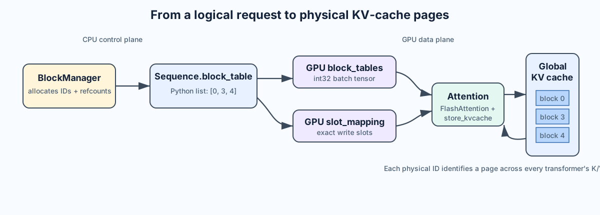
At initialization, ModelRunner allocates a cache with this shape:

[K/V, transformer layer, physical block, token offset in block,
 KV head local to this GPU rank, head dimension]

[2, L, N, block_size, H_kv_per_rank, D]

2 distinguishes keys from values. L is the number of transformer layers and N is the number of physical blocks the current GPU can support. The runner assigns each attention layer a view of its own slice:

layer i: k_cache = kv_cache[0, i]
         v_cache = kv_cache[1, i]

That means physical block ID 7 is a 4-token page across every layer’s K and V cache in the toy example. The same ID appears in each layer’s local k_cache/v_cache, but at that layer’s slice.

1.1 How the cache pool size is chosen

Each rank starts in a fixed order: initialize the NCCL process group, select its CUDA device, create and load its Qwen3 model shard, create a sampler, warm up the model without KV pages, allocate the KV-cache pool, and (unless eager mode is forced) capture decode CUDA graphs. The physical cache pool is allocated once, after weights load and warm-up. Its per-block byte size is:

block_bytes = 2                         # K and V
            × L                         # transformer layers
            × block_size
            × H_kv_per_rank
            × D                         # head dimension
            × bytes_per_element         # e.g. 2 for fp16/bf16

The runner queries CUDA memory statistics, applies gpu_memory_utilization, computes how many such blocks fit, and then calls one torch.empty(...) to allocate the global cache. Larger models need more cache bytes per token because they have more layers, more KV heads, a larger head dimension, or a wider dtype. Tensor parallelism reduces H_kv_per_rank, so each rank owns a smaller shard of the KV cache.

The allocation in ModelRunner.allocate_kv_cache() expresses both the capacity calculation and the permanent tensor shape:

free, total = torch.cuda.mem_get_info()
used = total - free
peak = torch.cuda.memory_stats()["allocated_bytes.all.peak"]
current = torch.cuda.memory_stats()["allocated_bytes.all.current"]
num_kv_heads = hf_config.num_key_value_heads // self.world_size
head_dim = getattr(hf_config, "head_dim", hf_config.hidden_size // hf_config.num_attention_heads)
block_bytes = 2 * hf_config.num_hidden_layers * self.block_size * num_kv_heads * head_dim * hf_config.dtype.itemsize
config.num_kvcache_blocks = int(total * config.gpu_memory_utilization - used - peak + current) // block_bytes
self.kv_cache = torch.empty(2, hf_config.num_hidden_layers, config.num_kvcache_blocks,
                            self.block_size, num_kv_heads, head_dim)

This is dynamic at initialization, not on every request. At runtime, the tensor does not grow or shrink. What changes dynamically is the set of IDs that the BlockManager marks free or used. Returning an ID to free_block_ids makes that region reusable; it does not return GPU memory to PyTorch or the operating system.

1.2 GPU memory, not “moving the cache into L1/L2”

The cache tensor is in GPU global memory—HBM on many data-center GPUs, but GDDR on GPUs such as the RTX 4070 Laptop used in the repository’s benchmark. FlashAttention does not migrate the long-lived KV cache into L1 or L2 as a separate cache-management operation. Its kernels tile portions of Q, K, and V through on-chip SRAM/registers while they compute attention, reducing expensive global-memory traffic. The persistent KV cache remains in GPU global memory.

2. A complete prefill trace: allocation, prefix sharing, and KV writes

BlockManager maintains a small CPU-side directory:

blocks[block_id]       -> {ref_count, hash, token_ids}
free_block_ids         -> IDs available for allocation
used_block_ids         -> IDs referenced by at least one live sequence
hash_to_block_id       -> full-prefix hash -> physical block ID

The Block metadata does not contain a copy of K and V tensors. It contains enough bookkeeping to decide whether a sequence may use a page of the global GPU cache.

2.1 Prompt A: allocate new pages

Let block_size = 4 and begin with eight free blocks:

free_block_ids = [0, 1, 2, 3, 4, 5, 6, 7]
used_block_ids = {}
hash_to_block_id = {}

Prompt A has eleven token IDs. We use small IDs so the page boundaries are visible:

A = [11, 12, 13, 14 | 21, 22, 23, 24 | 31, 32, 33]
      logical page 0     logical page 1     logical page 2 (partial)

A.num_blocks = ceil(11 / 4) = 3. The scheduler calls:

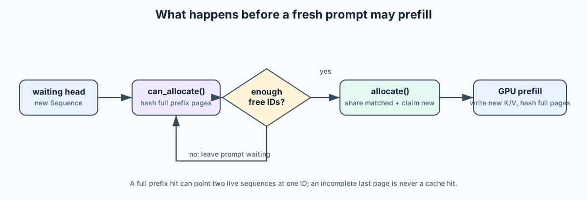
num_cached_blocks = block_manager.can_allocate(A)
block_manager.allocate(A, num_cached_blocks)

can_allocate() looks only for reusable complete logical pages. It checks range(seq.num_blocks - 1), so the final partial page is never considered a prefix-cache hit. For A, the hash table is empty, so it returns 0 after confirming that three free IDs are available.

This is the critical logic in BlockManager.can_allocate():

h = -1
num_cached_blocks = 0
num_new_blocks = seq.num_blocks
for i in range(seq.num_blocks - 1):
    token_ids = seq.block(i)
    h = self.compute_hash(token_ids, h)
    block_id = self.hash_to_block_id.get(h, -1)
    if block_id == -1 or self.blocks[block_id].token_ids != token_ids:
        break
    num_cached_blocks += 1
    if block_id in self.used_block_ids:
        num_new_blocks -= 1

if len(self.free_block_ids) < num_new_blocks:
    return -1
return num_cached_blocks

allocate(A, 0) takes three IDs from the free deque:

A.block_table = [0, 1, 2]

physical block 0 <- logical page A0: [11, 12, 13, 14]
physical block 1 <- logical page A1: [21, 22, 23, 24]
physical block 2 <- logical page A2: [31, 32, 33]

ref_count(0, 1, 2) = (1, 1, 1)
free_block_ids = [3, 4, 5, 6, 7]
used_block_ids = {0, 1, 2}

This table does not yet say that cache values have been calculated. It merely reserves the locations into which the next model forward pass will write them.

The allocation phase shares the matching prefix IDs first, then claims IDs for the remaining pages (BlockManager.allocate()):

for i in range(num_cached_blocks):
    token_ids = seq.block(i)
    h = self.compute_hash(token_ids, h)
    block_id = self.hash_to_block_id[h]
    block = self.blocks[block_id]
    if block_id in self.used_block_ids:
        block.ref_count += 1
    else:
        block.ref_count = 1
        self.free_block_ids.remove(block_id)
        self.used_block_ids.add(block_id)
    seq.block_table.append(block_id)

for _ in range(num_cached_blocks, seq.num_blocks):
    seq.block_table.append(self._allocate_block())

seq.num_cached_tokens = num_cached_blocks * self.block_size

2.2 How a logical position becomes a GPU cache slot

For a position p in a sequence, the CPU-side lookup is:

logical_page = p // block_size
offset       = p % block_size
physical_id  = seq.block_table[logical_page]
slot         = physical_id * block_size + offset

For A, position 6 is token 23:

logical_page = 6 // 4 = 1
offset       = 6 % 4 = 2
physical_id  = A.block_table[1] = 1
slot         = 1 * 4 + 2 = 6

The slot is a flattened location in this rank’s [N, block_size, H_kv_per_rank, D] layer cache. A real block table can be fragmented. If another sequence uses [0, 4, 7], its position 6 maps to physical page 4, offset 2, so slot 4 * 4 + 2 = 18. Logical positions remain contiguous even though physical pages do not.

ModelRunner.prepare_prefill() constructs precisely those flattened slot IDs for the scheduled range:

start = seq.num_cached_tokens
end = start + seq.num_scheduled_tokens
start_block = start // self.block_size
end_block = (end + self.block_size - 1) // self.block_size
for i in range(start_block, end_block):
    slot_start = seq.block_table[i] * self.block_size
    if i == start_block:
        slot_start += start % self.block_size
    if i != end_block - 1:
        slot_end = seq.block_table[i] * self.block_size + self.block_size
    else:
        slot_end = seq.block_table[i] * self.block_size + end - i * self.block_size
    slot_mapping.extend(range(slot_start, slot_end))

This is the real branch: the first-page adjustment and final-page boundary keep the mapping aligned with exactly the scheduled token range.

2.3 ModelRunner turns A’s metadata into GPU inputs

For an initial, full prefill of A:

num_cached_tokens = 0
num_scheduled_tokens = 11
start = 0, end = 11

prepare_prefill() builds:

input_ids     = [11, 12, 13, 14, 21, 22, 23, 24, 31, 32, 33]
positions     = [ 0,  1,  2,  3,  4,  5,  6,  7,  8,  9, 10]
cu_seqlens_q  = [0, 11]
cu_seqlens_k  = [0, 11]
slot_mapping  = [0, 1, 2, 3, 4, 5, 6, 7, 8, 9, 10]

cu_seqlens_q is the cumulative length of packed query tokens; cu_seqlens_k is the cumulative attention-context length. With a single fresh prompt they are the same. The batch has no cached prefix, so no GPU block_tables tensor is needed for the prefill attention read: the K/V values for all 11 tokens are already present as the packed K/V tensors calculated in this same forward pass.

The attention layer nevertheless writes newly calculated keys and values to the global cache. Its Triton store_kvcache kernel receives slot_mapping; entry j tells it where the K and V vectors of packed token j belong. In outline:

if k_cache.numel() and v_cache.numel():
    store_kvcache(k, v, k_cache, v_cache, context.slot_mapping)

That is the cache-write gate in Attention.forward(); the attention branch that follows chooses the prefill or decode kernel using the same per-step context.

for every transformer layer:
    calculate K and V for A's 11 input tokens
    write K/V for token j into [physical slot_mapping[j]]

The attention layer then uses flash_attn_varlen_func for causal prompt attention. After this forward pass, A’s physical pages contain real KV values across every transformer layer.

2.4 Hash full pages after the successful run

Only after model execution does Scheduler.postprocess() call hash_blocks(A). At this instant, num_cached_tokens = 0 and num_scheduled_tokens = 11, so:

start = 0 // 4 = 0
end   = 11 // 4 = 2

It hashes physical blocks 0 and 1, but not partial physical block 2:

h0 = H([11, 12, 13, 14])
h1 = H(previous_hash=h0, [21, 22, 23, 24])

hash_to_block_id[h0] = 0
hash_to_block_id[h1] = 1

The hash is incremental: page 1’s key includes the hash of all prior full pages. Thus a page with identical tokens in a different earlier context does not accidentally become the same prefix-cache entry. The metadata also saves the token IDs and checks them on lookup, avoiding a hash-only decision.

The scheduler then records that all 11 prompt tokens are cached and appends the first sampled completion token. That sampled token has not yet had its own K/V vectors calculated; the next decode pass will do that.

2.5 Prompt B: reuse A’s first page and calculate only its suffix

Now add a second request:

B = [11, 12, 13, 14 | 51, 52, 53, 54 | 61, 62, 63, 64 | 71]
      same as A page 0   different page 1      page 2       partial page 3

B has 13 tokens and four pages. can_allocate(B) proceeds as follows:

1. Hash B’s first page. It finds h0 -> physical block 0; the saved IDs match.
2. It increments num_cached_blocks to 1.
3. Block 0 is already in used_block_ids because A is still live, so B can share it without consuming a new free ID. num_new_blocks falls from 4 to 3.
4. It hashes B’s second page using h0 as its prefix. It does not match A’s page 1, so prefix matching stops.
5. It verifies that at least three IDs are free and returns 1.

Then allocate(B, 1) produces:

B.block_table = [0, 3, 4, 5]

block 0: shared with A; ref_count 1 -> 2
block 3: B's [51, 52, 53, 54]
block 4: B's [61, 62, 63, 64]
block 5: B's [71]

B.num_cached_tokens = 1 * 4 = 4

There is a subtle branch worth knowing. A hash entry may point to a free block left behind by a completed request. In that case allocate() removes the ID from free_block_ids, puts it back in used_block_ids, and sets its reference count to 1. In can_allocate(), such a reuse does not reduce the number of free pages required, because the block must be claimed from the free pool. A live shared block does reduce the requirement.

For B’s prefill, the runner processes only the uncached suffix:

start = 4, end = 13
input_ids    = [51, 52, 53, 54, 61, 62, 63, 64, 71]
positions    = [ 4,  5,  6,  7,  8,  9, 10, 11, 12]
cu_seqlens_q = [0, 9]       # nine new query tokens
cu_seqlens_k = [0, 13]      # attention sees the 4-token prefix too
slot_mapping = [12, 13, 14, 15, 16, 17, 18, 19, 20]
block_tables = [[0, 3, 4, 5]]  # int32 GPU tensor in the real code

The slots are 12–15 for page 3, 16–19 for page 4, and 20 for page 5. The attention module first writes B’s new K/V vectors into those slots. Because cu_seqlens_k is longer than cu_seqlens_q, it then passes the GPU block table to FlashAttention. The kernel can read A/B’s shared prefix from physical block 0 and B’s just-written suffix from pages 3–5, as if B had one logically contiguous 13-token context.

Postprocessing hashes B’s newly complete pages only:

start = 4 // 4 = 1
end   = 13 // 4 = 3

hash B logical pages 1 and 2 -> physical blocks 3 and 4
do not hash partial physical block 5 yet

This is prefix caching in its complete form: scheduling avoids recomputing an existing prefix, metadata maps the request to its physical pages, and GPU attention consumes those pages without making the cache contiguous.

3. Decode, page growth, and logical release

Decode is slightly counterintuitive because its input token is the completion token sampled by the preceding model call. That token exists in seq.token_ids, but its K/V state does not exist until decode processes it.

3.1 A crosses a page boundary

Return to A. Its 11-token prompt yielded first completion token 99, so the sequence now contains 12 tokens:

A = [11, 12, 13, 14 | 21, 22, 23, 24 | 31, 32, 33, 99]
A.block_table = [0, 1, 2]

The scheduler asks can_append(A) before decode. The code is:

def can_append(self, seq):
    return len(self.free_block_ids) >= (len(seq) % self.block_size == 1)

def may_append(self, seq):
    if len(seq) % self.block_size == 1:
        seq.block_table.append(self._allocate_block())

At length 12, 12 % 4 != 1, so no new physical page is needed. Decode will process 99, which belongs in existing page 2 at offset 3. prepare_decode() creates:

input_ids    = [99]
positions    = [11]
context_lens = [12]
slot_mapping = [2 * 4 + 3] = [11]
block_tables = [[0, 1, 2]]

flash_attn_with_kvcache writes K/V for 99 to slot 11 and attends over A’s 12-token history. The sampler returns a next token, say 100. Before postprocess() appends 100, hash_blocks() can now hash the full third page [31, 32, 33, 99].

After appending 100, A has length 13. On its next decode scheduling turn, 13 % 4 == 1, which means its current last token is the first token in a new logical page. The scheduler must reserve a new page before processing it:

may_append(A) allocates physical block 6
A.block_table becomes [0, 1, 2, 6]

decode input: 100
position:     12
slot:         6 * 4 + 0 = 24

The apparent == 1 condition is correct once the timing is clear: the output token was appended after the previous call; the next decode will calculate that token’s KV state. It needs a new page exactly when that already-appended token is the first token of a page.

3.2 Why decode needs both a slot mapping and a block table

For each request in a decode batch, slot_mapping identifies one write position: where this request’s last input token stores its newly calculated K/V values. block_tables identifies all pages belonging to the request: where attention reads the entire history.

For example, two active requests with different page layouts become a padded GPU tensor:

A.block_table = [0, 1, 2, 6]
B.block_table = [0, 3, 4, 5]

prepare_block_tables([A, B])
  -> [[0, 1, 2, 6],
      [0, 3, 4, 5]]

If one row were shorter, prepare_block_tables() would pad it with -1. Each attention kernel also receives context lengths, so it knows how much of the logical history is valid. The values are copied from CPU Python lists to pinned host tensors and then asynchronously transferred to the GPU; pin_memory=True and cuda(non_blocking=True) make that small host-to-device transfer efficient.

3.3 Completion and preemption release IDs, not the global tensor

When A finishes, deallocate(A) walks its IDs in reverse. Suppose block 0 is shared with B:

A.block_table before finish = [0, 1, 2, 6]

block 6: ref_count 1 -> 0; return ID 6 to free_block_ids
block 2: ref_count 1 -> 0; return ID 2
block 1: ref_count 1 -> 0; return ID 1
block 0: ref_count 2 -> 1; keep it used for B

Only when B later releases block 0 does its count fall to zero and the ID return to the free deque. The K/V bytes can stay physically present in the GPU tensor even after that. They are simply no longer owned by a live sequence. The hash metadata may also remain, permitting a later exact-prefix request to reclaim the page; _allocate_block() removes a stale hash entry only when it repurposes that page for unrelated content.

Preemption uses the same deallocate() path. It frees logical pages immediately, moves the sequence back to waiting, clears its block table and cached-token count, and requires later prefill/recomputation. It is not GPU-memory eviction to CPU RAM and it is not lossless suspension.

4. ModelRunner.run(): from scheduled sequences to sampled token IDs

The method that LLMEngine.step() invokes is short:

This is the complete ModelRunner.run() control path:

def run(self, seqs, is_prefill):
    input_ids, positions = self.prepare_prefill(seqs) if is_prefill else self.prepare_decode(seqs)
    temperatures = self.prepare_sample(seqs) if self.rank == 0 else None
    logits = self.run_model(input_ids, positions, is_prefill)
    token_ids = self.sampler(logits, temperatures).tolist() if self.rank == 0 else None
    reset_context()
    return token_ids

prepare_prefill() and prepare_decode() do not initialize the Python Sequence.block_table. That happened earlier in BlockManager.allocate() or BlockManager.may_append(). The runner serializes the already-decided mapping into GPU-friendly tensors and stores them in a process-local Context. Attention.forward() reads that context when the model reaches every transformer layer.

4.1 Packed prefill batch: why there are two cumulative-length arrays

Consider a prefill batch after prefix caching:

C: 4 cached tokens + 3 scheduled tokens
D: 0 cached tokens + 2 scheduled tokens

The packed model input contains only the five scheduled token IDs:

input_ids    = [C4, C5, C6, D0, D1]
positions    = [ 4,  5,  6,  0,  1]
cu_seqlens_q = [0, 3, 5]
cu_seqlens_k = [0, 7, 9]

cu_seqlens_q says “the first packed query occupies rows 0–2; the second occupies rows 3–4.” cu_seqlens_k says “C attends to a logical 7-token context and D to a logical 2-token context.” The difference for C tells the prefill attention kernel that a block table is necessary to find its cached first four tokens.

The runner’s set_context(...) is not a distributed database or persistent request state. It is simply a module-level Python object holding these tensors during one forward pass. reset_context() clears it immediately afterward.

prepare_sample() is intentionally much simpler. For a decode batch with temperatures 0.8 and 1.0, it creates the GPU tensor tensor([0.8, 1.0], dtype=float32). Rank 0 passes it to Sampler, so each request can use its own temperature even though the requests share one model forward pass.

4.2 Eager prefill versus CUDA-graph decode

Prefill has variable token counts and packed shapes, so nano-vLLM runs it eagerly. Decode has a more regular shape—one input token per live sequence—and can benefit from CUDA Graphs.

A CUDA Graph records a fixed sequence of GPU launches, dependencies, and memory addresses. Replaying it removes much of Python/CPU kernel-launch overhead, which matters when each decode step otherwise performs tiny amounts of work. It does not precompute a token answer; before replay, the runner copies the current token IDs, positions, slot mapping, context lengths, and block tables into fixed graph input buffers.

At initialization, capture_cudagraph() prepares fixed buffers and records graphs for batch sizes:

1, 2, 4, 8, 16, 32, ... up to min(max_num_seqs, 512)

For an actual decode batch of three sequences, run_model() chooses the size-4 graph, fills the first three entries of its static buffers, replays it, and returns the first three hidden states to the language-model head. It uses eager execution instead when enforce_eager=True, for prefill, or for a decode input containing more than 512 rows.

The CUDA-graph branch is small but revealing (ModelRunner.run_model()):

graph = self.graphs[next(x for x in self.graph_bs if x >= bs)]
graph_vars = self.graph_vars
graph_vars["input_ids"][:bs] = input_ids
graph_vars["positions"][:bs] = positions
graph_vars["slot_mapping"].fill_(-1)
graph_vars["slot_mapping"][:bs] = context.slot_mapping
graph_vars["context_lens"].zero_()
graph_vars["context_lens"][:bs] = context.context_lens
graph_vars["block_tables"][:bs, :context.block_tables.size(1)] = context.block_tables
graph.replay()
return self.model.compute_logits(graph_vars["outputs"][:bs])

This constraint explains the seemingly fussy preparation code: CUDA Graph replay needs stable buffer addresses and supported tensor shapes, while the values inside those buffers change every token.

5. Multi-GPU execution: worker processes, shared control messages, and NCCL

With tensor_parallel_size=1, the model runner uses one process and one CUDA device. With tensor_parallel_size=K, LLMEngine starts K - 1 worker processes, one for ranks 1 through K - 1, and creates rank 0 in the original process.

The setup loop in LLMEngine.__init__() makes the ownership concrete:

for i in range(1, config.tensor_parallel_size):
    event = ctx.Event()
    process = ctx.Process(target=ModelRunner, args=(config, i, event))
    process.start()
    self.ps.append(process)
    self.events.append(event)
self.model_runner = ModelRunner(config, 0, self.events)

main process / rank 0 / GPU 0
  ├── worker process / rank 1 / GPU 1
  ├── worker process / rank 2 / GPU 2
  └── ...

world_size is the total number of participating processes/GPU ranks. rank is one process’s integer identity in 0 .. world_size - 1. Every rank initializes a torch.distributed process group using NCCL and calls torch.cuda.set_device(rank). These worker processes are not CPU-only helpers: each owns a GPU, builds a model shard, allocates a local KV-cache shard, and executes every forward pass.

5.1 What the events and shared-memory buffer do

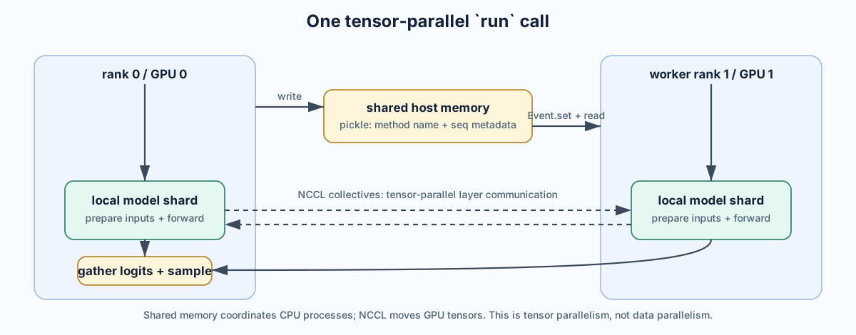
The rank-0 process creates one multiprocessing.Event per worker and a named 1 MiB SharedMemory segment called nanovllm. Shared memory here means an operating-system shared region in host RAM mapped into multiple processes; it is not a disk file and it is not GPU memory.

When rank 0 calls:

self.model_runner.call("run", seqs, is_prefill)

it performs the following control-plane protocol:

1. pickle ["run", seqs, is_prefill]
2. write its byte length to shared-memory bytes 0:4
3. write the pickle payload after that header
4. set every worker's Event
5. execute rank 0's own run(seqs, is_prefill)

each worker:
6. wakes from Event.wait()
7. reads length and payload from shared memory
8. unpickles the method name and Sequence metadata
9. dispatches getattr(self, "run")(...)

The same mechanism sends exit. It is a compact control channel that makes every rank run the same method with the same sequence metadata. It is not how large activation tensors or the KV cache move between GPUs; the fixed 1 MiB buffer is also a practical limitation of this teaching implementation.

Rank 0’s ModelRunner.write_shm() and call() write only the small control payload, signal workers, then run the local method:

data = pickle.dumps([method_name, *args])
n = len(data)
self.shm.buf[0:4] = n.to_bytes(4, "little")
self.shm.buf[4:n + 4] = data
for event in self.event:
    event.set()

def call(self, method_name, *args):
    if self.world_size > 1 and self.rank == 0:
        self.write_shm(method_name, *args)
    method = getattr(self, method_name, None)
    return method(*args)

5.2 What tensor parallelism does during the forward pass

Each rank receives its own GPU copies of the small inputs (input_ids, positions, cache metadata) and runs the model concurrently. The model’s parallel linear layers shard weights by rank. In the Qwen3 attention path, the Q/K/V projection is column-parallel, so each rank owns a subset of attention and KV heads. Row-parallel output projections use NCCL all_reduce to combine partial results. Similar sharding appears in the MLP and vocabulary head.

Therefore, the data plane is:

Shared memory + Events:    CPU control message: "run this batch"
per-rank GPU tensors:      local inputs and local KV-cache shard
NCCL collectives:          GPU-to-GPU communication for tensor-parallel layers
rank 0 sampler:            select the next token IDs returned to the scheduler

The vocabulary-parallel language-model head gathers its per-rank vocabulary-logit shards to rank 0, so rank 0 has the full logits and performs sampling; workers return None from run(). The scheduler and postprocessing remain in the original process, so there is one authoritative set of Sequence objects and block-manager metadata.

This is intentionally straightforward multiprocessing. Production tensor-parallel serving needs more robust rendezvous configuration, error propagation, request cancellation, command framing, memory isolation, and worker health handling than this example provides.

6. The durable mental model

The CPU and GPU sides are connected by stable IDs, not by copying a per-request KV cache around:

1. ModelRunner allocates one global, per-rank GPU KV-cache pool at startup.
2. Scheduler + BlockManager assign/reuse integer block IDs for each Sequence.
3. ModelRunner converts those Python lists to GPU block-table tensors and slot mappings.
4. Every attention layer writes new K/V vectors to the mapped slots and reads the
   request's old pages through the same mapping.
5. Hashes and reference counts allow full prefix pages to be shared safely.
6. Completion or preemption returns IDs to the pool; the preallocated tensor stays.

Part 3 will move inside the neural computation itself: QKV projection, RoPE, RMSNorm, FlashAttention, token sampling, and the optimizations that make these small operations fast enough to matter.