nano-vLLM Part 3: Qwen3, Tensor Parallelism, and One Forward Pass

Part 1 followed the scheduler. Part 2 followed its block IDs into the per-rank KV cache. This post enters the model call itself: once ModelRunner has prepared input_ids, positions, slot mappings, and block tables, what Qwen3 model runs on each GPU—and when do GPUs actually communicate?

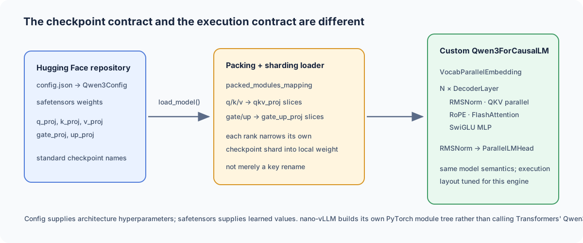
The short answer is easy to state but worth unpacking: nano-vLLM reads a Hugging Face Qwen3 configuration and checkpoint, but it does not instantiate Transformers’ Qwen3 implementation for its forward pass. It builds its own small PyTorch module tree from qwen3.py and custom layers. That lets the implementation choose fused checkpoint layouts, tensor-parallel weight sharding, paged-KV-cache attention, and a narrow sampling path.

The central source files are qwen3.py, linear.py, embed_head.py, rotary_embedding.py, and loader.py. As in the earlier posts, the code discussed is the repository’s main branch at the time of writing.

1. One model, two compatible contracts

1.1 Hugging Face provides the model description and learned values

The Hugging Face repository supplies two different things:

config.json, which becomes Qwen3Config and tells nano-vLLM architectural facts such as vocabulary size V, hidden size H, layer count, attention-head count, KV-head count, RoPE settings, and MLP intermediate size I;
.safetensors files, which contain the learned checkpoint tensors under names such as q_proj.weight, k_proj.weight, v_proj.weight, gate_proj.weight, and up_proj.weight.

nano-vLLM uses those inputs to construct a different execution layout. This is not converting the model’s learned function into a different model; it is adapting the representation of the same learned matrices to an inference-oriented module tree.

Hugging Face checkpoint contract and nano-vLLM execution contract

The top-level model is compact:

class Qwen3ForCausalLM(nn.Module):
    def __init__(self, config):
        super().__init__()
        self.model = Qwen3Model(config)
        self.lm_head = ParallelLMHead(config.vocab_size, config.hidden_size)
        if config.tie_word_embeddings:
            self.lm_head.weight.data = self.model.embed_tokens.weight.data

    def forward(self, input_ids, positions):
        return self.model(input_ids, positions)

    def compute_logits(self, hidden_states):
        return self.lm_head(hidden_states)

Qwen3ForCausalLM deliberately separates the transformer body from compute_logits(). The body returns hidden states; the language-model head turns them into one score per vocabulary token. When embeddings are tied, each rank’s output-head weight aliases that rank’s input-embedding shard instead of allocating a second local copy.

At tensor_parallel_size = 1, these custom modules still work: every shard is the whole relevant tensor and branches guarded by tp_size > 1 do no inter-GPU collective. The value of the custom implementation is not only multi-GPU support, though. It also supplies the paged-cache attention interface and simple compiled operations that the generic Transformers forward path does not use in this shape.

1.2 The complete custom model/layer inventory

At the time of writing, nano-vLLM has one architecture-specific model implementation: Qwen3. The following inventory covers the model file and every module in its layers/ directory. “Custom” here means implemented by nano-vLLM; it does not mean every operation is handwritten CUDA.

Source file	Custom component(s)	Runtime responsibility
`models/qwen3.py`	`Qwen3ForCausalLM`, `Qwen3Model`, `Qwen3DecoderLayer`, `Qwen3Attention`, `Qwen3MLP`	Qwen3 model structure: embedding, repeated pre-norm decoder blocks, final norm, and vocabulary logits
`layers/linear.py`	`LinearBase`, `ReplicatedLinear`, `ColumnParallelLinear`, `MergedColumnParallelLinear`, `QKVParallelLinear`, `RowParallelLinear`	Store/load TP weight shards; run local linear operations; all-reduce row-parallel outputs
`layers/embed_head.py`	`VocabParallelEmbedding`, `ParallelLMHead`	Vocabulary-sharded input lookup and output-logit projection/gather
`layers/attention.py`	`Attention`, `store_kvcache`, `store_kvcache_kernel`	Interface to the paged per-rank KV cache, FlashAttention calls, and Triton KV writes
`layers/layernorm.py`	`RMSNorm`	RMS normalization and fused residual-add-plus-normalization path
`layers/rotary_embedding.py`	`RotaryEmbedding`, `get_rope`, `apply_rotary_emb`	Precompute RoPE tables and rotate Q/K at run time
`layers/activation.py`	`SiluAndMul`	The fused SwiGLU activation operation
`layers/sampler.py`	`Sampler`	Temperature-scaled categorical sampling on rank 0

ModelRunner is not a neural-network layer, but it is the runtime bridge: it creates Qwen3ForCausalLM, loads its checkpoint shards, builds the per-rank KV cache, prepares batch tensors, dispatches the forward call, and coordinates worker ranks. The scheduler, block manager, and sequence objects from Parts 1–2 are likewise custom engine components, rather than Qwen3 layers.

1.3 Fusing checkpoint modules is more than renaming a key

The standard checkpoint exposes Q, K, and V as separate projection tensors. nano-vLLM stores the corresponding local pieces adjacent in one qkv_proj parameter. It does the analogous thing for the two MLP input projections:

packed_modules_mapping = {
    "q_proj": ("qkv_proj", "q"),
    "k_proj": ("qkv_proj", "k"),
    "v_proj": ("qkv_proj", "v"),
    "gate_proj": ("gate_up_proj", 0),
    "up_proj": ("gate_up_proj", 1),
}

The mapping changes a checkpoint name to an internal destination name and supplies a shard identifier. In load_model(), that identifier is passed to the target parameter’s specialized loader:

for k in packed_modules_mapping:
    if k in weight_name:
        v, shard_id = packed_modules_mapping[k]
        param_name = weight_name.replace(k, v)
        param = model.get_parameter(param_name)
        weight_loader = getattr(param, "weight_loader")
        weight_loader(param, f.get_tensor(weight_name), shard_id)
        break

For example, on a two-rank run, the loader handles layers.0.self_attn.q_proj.weight as follows:

checkpoint key:     ...q_proj.weight                    [total_Q_width, H]
internal parameter: ...qkv_proj.weight                  [local_QKV_width, H]
shard ID:           "q"

1. take rank r's contiguous Q-head rows from the checkpoint tensor;
2. narrow the local fused QKV buffer to its Q region;
3. copy that rank-r Q slice into the region.

Then K and V fill the next two local regions. QKVParallelLinear.weight_loader() makes that placement explicit:

if loaded_shard_id == "q":
    shard_size, shard_offset = self.num_heads * self.head_size, 0
elif loaded_shard_id == "k":
    shard_size = self.num_kv_heads * self.head_size
    shard_offset = self.num_heads * self.head_size
else:
    shard_size = self.num_kv_heads * self.head_size
    shard_offset = self.num_heads * self.head_size + self.num_kv_heads * self.head_size
param_data = param_data.narrow(self.tp_dim, shard_offset, shard_size)
loaded_weight = loaded_weight.chunk(self.tp_size, self.tp_dim)[self.tp_rank]
param_data.copy_(loaded_weight)

narrow(dim, start, length) selects a contiguous view. Here it chooses a destination region in the local fused tensor; chunk(...)[rank] chooses this rank’s output-feature slice from the original checkpoint tensor. Therefore the mapping is not a harmless textual rename: it is the loader’s instruction for fuse, place, and shard.

Full vLLM supports far more architectures and parallelism strategies, so it needs a much larger compatibility layer: architecture-specific model implementations, weight-name conventions, quantized/packed formats, and parallelism-aware loaders. TensorRT-LLM has a related goal—make a trained model executable efficiently—but uses a different deployment pipeline and compilation/runtime model. Neither system can generally “automatically optimize any arbitrary Hugging Face Python model” without an architecture-aware implementation path.

1.4 Custom layout, `torch.compile`, Triton, FlashAttention, and CUDA Graphs are different layers of optimization

It is useful not to collapse all of nano-vLLM’s optimizations into the word “compile.” The project uses several distinct mechanisms:

Mechanism	In this repository	What it does
Custom PyTorch model/layout	Qwen3 classes, fused QKV/gate-up parameters, TP layer classes, custom loader	Defines the execution-compatible model and how checkpoint weights are placed into it
Standard PyTorch/GPU libraries	`F.linear`, embedding lookup, elementwise tensor operations	Dispatches ordinary GPU work through PyTorch’s backend; this is not a hand-written matrix-multiplication kernel
`torch.compile`	`RMSNorm` paths, `RotaryEmbedding.forward`, `SiluAndMul.forward`, `Sampler.forward`	Compiles selected PyTorch functions so their small sequences of operations can be optimized/fused
Triton	`store_kvcache_kernel`	Writes each new local K/V vector into its paged-cache slot
FlashAttention package	prefill `flash_attn_varlen_func`, decode `flash_attn_with_kvcache`	Runs the specialized attention kernels over packed prompt tensors or the paged cache
CUDA Graphs	captured by `ModelRunner` for supported decode batch sizes	Replays a fixed GPU-launch graph to reduce decode launch overhead; see Part 2

This is therefore not a TensorRT-LLM-style ahead-of-time engine build that lowers the full model into one standalone runtime artifact. nano-vLLM remains a PyTorch program, but it arranges its model and hot operations so PyTorch, TorchInductor, Triton, FlashAttention, NCCL, and CUDA Graphs can each handle the narrow piece they are good at.

2. A concrete tensor-parallel forward pass

To make shapes visible, use this intentionally tiny two-GPU model:

TP = 2, vocabulary V = 32, hidden size H = 8
Q heads = 4, KV heads = 2, head dimension D = 2
MLP intermediate size I = 16, packed tokens in this call T = 5

This is a teaching model, not a claim about a particular released Qwen3 checkpoint. Each rank owns 16 vocabulary rows, 2 query heads, 1 KV head, and 8 MLP intermediate features. The same logic applies to real dimensions.

ModelRunner produces inputs differently for prefill and decode, but the model interface is identical:

Stage	`input_ids` and `positions` per rank	Meaning
Prefill	packed `[T]`, e.g. five newly scheduled prompt tokens	one row per new prompt token; positions may be nonzero with prefix reuse
Decode	`[B]`, one `seq.last_token` per selected request	one already-sampled token per live sequence; its position is `len(seq) - 1`

Rank 0 sends run(seqs, is_prefill) to worker processes as described in Part 2. Each rank then independently prepares the same small input_ids, positions, and cache metadata on its own GPU. The inputs are replicated; the large parameter matrices and KV cache are mostly sharded. A module hierarchy exists on every rank, but that does not mean every rank stores a full copy of every parameter:

vocabulary embedding and language-head rows are vocabulary-sharded;
QKV and MLP expansion outputs are column-parallel shards;
attention output and MLP down-projection inputs are row-parallel shards;
RMSNorm scale vectors and RoPE tables are replicated because they are small;
each rank owns a KV-cache shard containing only its local KV heads.

The same simple design imposes hard constraints. VocabParallelEmbedding asserts V % TP == 0; Qwen3Attention asserts both total query heads and total KV heads divide by TP; and the parallel linear helpers assert their sharded feature dimensions divide evenly too. A configuration with uneven head or vocabulary partitions is unsupported rather than load-balanced.

Each process constructs its own module tree and calls load_model() locally. It reads checkpoint tensors on the CPU, narrows/copies the rank’s destination shard into that process’s GPU parameters, and later synchronizes with the other ranks through its NCCL collectives and setup barrier. There is no shared GPU parameter allocation and no one-rank-load-then-broadcast optimization in this compact implementation. That simplicity is useful for reading the code, but it can duplicate checkpoint I/O and host-memory work compared with a production distributed loader.

The resulting communication rhythm is the important part.

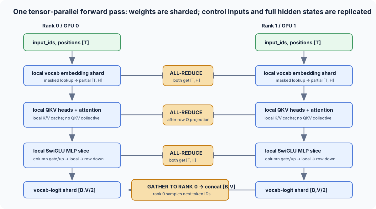
Tensor-parallel forward pass and collective boundaries

An all-reduce takes one same-shaped tensor from every rank, sums them elementwise, and leaves the summed tensor on every rank. In nano-vLLM, the process group is initialized with the nccl backend, so PyTorch’s dist.all_reduce() and dist.gather() are backed by NCCL GPU collectives. The older LLM Training Parallelism Basics post gives broader background on all-reduce, all-gather, and reduce-scatter; here the focus is the exact inference data flow.

2.1 Vocabulary-parallel embedding: shard weights, not requests

VocabParallelEmbedding does not route token 19 to a separate request queue on one GPU. Every rank receives every token ID; each rank checks whether it owns that ID, produces a nonzero vector only for tokens in its contiguous vocabulary range, and all-reduces the partial results.

For input IDs [2, 19, 30] in the toy model:

rank 0 vocabulary rows: [0, 16)     mask = [true,  false, false]
rank 1 vocabulary rows: [16, 32)    mask = [false, true,  true]

rank 0 partial [3, 8]: [E2, 0,   0]
rank 1 partial [3, 8]: [0,  E19, E30]
all_reduce on both ranks: [E2, E19, E30]   shape [3, 8]

The actual code is brief:

mask = (x >= self.vocab_start_idx) & (x < self.vocab_end_idx)
x = mask * (x - self.vocab_start_idx)
y = F.embedding(x, self.weight)
y = mask.unsqueeze(1) * y
dist.all_reduce(y)

The temporary lookup of local index zero for a non-owned token is harmless because the mask zeroes that output before the collective. Routing individual IDs would replace one regular collective with irregular token exchanges. This design trades replicated tiny ID tensors and a [T,H] all-reduce for simple, dense GPU execution. An embedding can certainly fit on one GPU for many models; vocabulary parallelism is used here because the implementation has a uniform tensor-parallel design and because vocabulary matrices become material at large V and H.

The result is available on all ranks, not only rank 0, because every later decoder-layer shard needs the same full hidden-state input.

3. One decoder layer: residual stream, local heads, and the first collective

Qwen3Model.forward() establishes the residual stream once, then threads it through every decoder layer:

hidden_states = self.embed_tokens(input_ids)
residual = None
for layer in self.layers:
    hidden_states, residual = layer(positions, hidden_states, residual)
hidden_states, _ = self.norm(hidden_states, residual)

The residual is None branch does not mean the first layer lacks a residual connection. It initializes the carried residual with the embedding output. The fused add-and-normalize path then takes over:

if residual is None:
    hidden_states, residual = self.input_layernorm(hidden_states), hidden_states
else:
    hidden_states, residual = self.input_layernorm(hidden_states, residual)
hidden_states = self.self_attn(positions, hidden_states)
hidden_states, residual = self.post_attention_layernorm(hidden_states, residual)
hidden_states = self.mlp(hidden_states)
return hidden_states, residual

For the first layer, the sequence is:

e = embedding(input_ids)
n0 = RMSNorm(e);                      residual = e
a  = Attention(n0)
n1, residual = RMSNorm(a + e);        residual = a + e
m  = MLP(n1)
return m, residual

At the next layer’s input norm, add_rms_forward(m, residual) forms m + (a + e), which is exactly the usual accumulated decoder output before the next attention sublayer. The implementation delays the addition until the next fused RMSNorm rather than materializing a separate residual-add tensor after every operation.

RMSNorm.add_rms_forward() performs the addition in float, saves the summed low-precision residual, then normalizes:

x = x.float().add_(residual.float())
residual = x.to(orig_dtype)
var = x.pow(2).mean(dim=-1, keepdim=True)
x.mul_(torch.rsqrt(var + self.eps))
x = x.to(orig_dtype).mul_(self.weight)

3.1 QKV is column-parallel; Q, K, and V are local

The first big matrix in attention is a fused QKVParallelLinear, a specialization of ColumnParallelLinear. In PyTorch a linear weight has shape [out_features, in_features]; despite the historical name, “column parallel” here means splitting the output-feature dimension across ranks. It takes the full [T,H] input on each rank and returns a different local output slice—no collective is necessary yet.

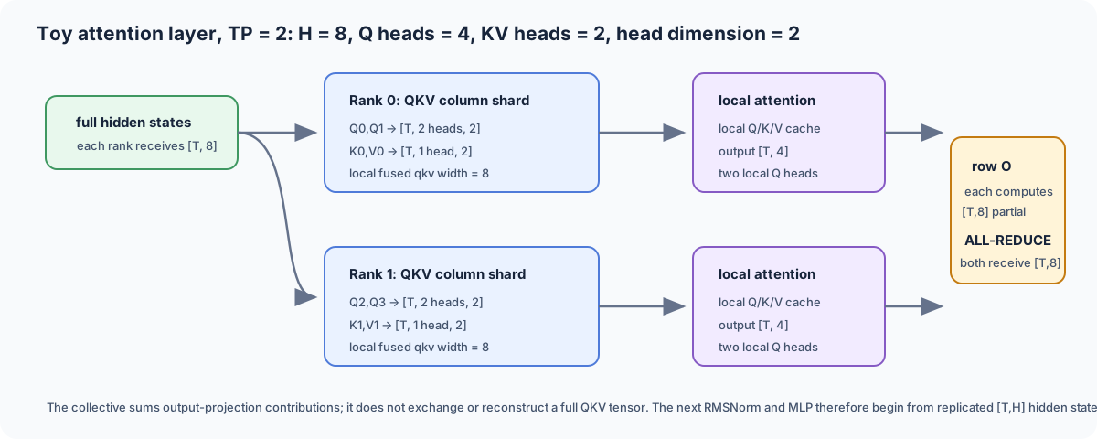
For the toy model, each rank starts with [5,8]. Its local QKV width is:

local Q width  = (4 query heads / 2 ranks) × D = 2 × 2 = 4
local K width  = (2 KV heads / 2 ranks) × D    = 1 × 2 = 2
local V width  = 2
local QKV width = 4 + 2 + 2 = 8

So each rank calculates qkv: [5,8], then splits and reshapes it into:

q: [5, 2, 2]       two local query heads
k: [5, 1, 2]       one local KV head
v: [5, 1, 2]       one local KV head

Having fewer KV heads than query heads is grouped-query attention (GQA): several query heads share each K/V head. It cuts KV-cache and attention bandwidth compared with one K/V head per query head. Those K/V tensors are written to the local rank’s paged cache; Part 2 explains how the per-rank block table and slot mapping identify the physical cache slots.

QKV and output-projection sharding with two ranks

The exact model forward sequence is:

qkv = self.qkv_proj(hidden_states)
q, k, v = qkv.split([self.q_size, self.kv_size, self.kv_size], dim=-1)
q = q.view(-1, self.num_heads, self.head_dim)
k = k.view(-1, self.num_kv_heads, self.head_dim)
v = v.view(-1, self.num_kv_heads, self.head_dim)
if not self.qkv_bias:
    q = self.q_norm(q)
    k = self.k_norm(k)
q, k = self.rotary_emb(positions, q, k)
o = self.attn(q, k, v)
output = self.o_proj(o.flatten(1, -1))

qkv_bias comes from the model configuration. If it is true, the local fused linear includes an equally sharded bias. If it is false, this particular implementation also creates and applies per-head Q/K RMSNorm. The code establishes that configuration coupling; it does not, by itself, prove a general rule that “a projection bias replaces Q/K normalization.” The important operational fact is their order: local Q/K normalization, then RoPE on Q/K, then local attention. V is neither Q/K-normalized here nor RoPE-rotated.

RoPE preserves shape. For head dimension D, it splits the final dimension into pairs and applies position-dependent 2D rotations to Q and K. The cache precomputes cosines and sines up to max_position:

inv_freq = 1.0 / (base**(torch.arange(0, rotary_dim, 2) / rotary_dim))
freqs = torch.einsum("i,j -> ij", t, inv_freq)
cache = torch.cat((freqs.cos(), freqs.sin()), dim=-1).unsqueeze_(1)

At run time it indexes the table with the supplied positions and rotates each local head independently. @lru_cache(1) caches the RotaryEmbedding module construction; it does not mean positions or Q/K values are reused across requests. rope_scaling can change the configured base used at construction, but this small implementation does not dynamically alter angles on every long decode step. For the underlying architecture—pre-norm/RMSNorm, SwiGLU, RoPE, QK normalization, and GQA—see LLM Architectures and Hyperparameters.

3.2 What the all-reduce does—and does not—communicate

Attention runs independently on each rank’s heads and rank-local K/V cache. For prefill it uses packed variable-length FlashAttention; for decode it uses flash_attn_with_kvcache. It writes new K/V values using slot_mapping in both cases. There is no all-reduce that reconstructs a global QKV tensor. For the algorithmic/kernel reason FlashAttention tiles K/Q/V and uses online softmax rather than materializing an attention matrix, see GPU Performance and Optimization. For the GPU execution and Triton background behind custom kernels such as nano-vLLM’s KV-cache store, see GPU Kernels & Triton Programming and Triton Introduction.

The first attention collective happens only after local attention output is flattened and fed to o_proj, a RowParallelLinear. Row parallel means the input-feature dimension of its weight is split. Each rank owns a weight [H, H / TP], consumes its local head slice [T, H / TP], and forms a complete-width partial contribution [T,H]. The contributions are then summed:

def forward(self, x):
    y = F.linear(x, self.weight, self.bias if self.tp_rank == 0 else None)
    if self.tp_size > 1:
        dist.all_reduce(y)
    return y

In the toy example, each rank sends a [5,8] partial output to the all-reduce and receives a [5,8] sum. It is not receiving another rank’s QKV matrix; it receives the completed attention hidden-state contribution. The bias is used only on rank 0 before summation so it is added once, not once per rank. That replicated [T,H] result feeds post-attention RMSNorm and the MLP on every rank.

4. The MLP repeats the same communication pattern

Qwen3MLP is a SwiGLU-style feed-forward block:

self.gate_up_proj = MergedColumnParallelLinear(
    hidden_size, [intermediate_size] * 2, bias=False)
self.down_proj = RowParallelLinear(intermediate_size, hidden_size, bias=False)

gate_up = self.gate_up_proj(x)
x = self.act_fn(gate_up)
x = self.down_proj(x)

The fused first projection avoids two separate reads of the same [T,H] input. It produces adjacent local gate and up pieces. SiluAndMul then implements the activation in exactly the expected order:

x, y = x.chunk(2, -1)
return F.silu(x) * y

For the toy dimensions, each rank receives the full [5,8] hidden state after attention. The column-parallel fused projection returns [5, 2I/TP] = [5,16]. The activation splits it into two [5,8] local pieces and returns [5,8] = [T,I/TP]. The row-parallel down projection turns that local input into one [5,8] partial hidden-state contribution, then all-reduces it. Thus every decoder layer has two main all-reduce boundaries:

full [T,H]
  → local attention heads → row O projection → ALL-REDUCE → full [T,H]
  → local SwiGLU features → row down projection → ALL-REDUCE → full [T,H]

This is why it is accurate to say that the MLP is “distributed again” after attention, but inaccurate to say that GPUs exchange a complete QKV tensor. Full hidden states are deliberately replicated at the start of each column-parallel phase; the expensive feature/head work and its weights stay partitioned.

4.1 Language-model head: gather, do not all-reduce

After the final RMSNorm, ParallelLMHead uses the vocabulary shards in the reverse direction from embedding. Each rank computes logits for only its local vocabulary rows:

if context.is_prefill:
    last_indices = context.cu_seqlens_q[1:] - 1
    x = x[last_indices].contiguous()
logits = F.linear(x, self.weight)
if self.tp_size > 1:
    all_logits = [torch.empty_like(logits) for _ in range(self.tp_size)] if self.tp_rank == 0 else None
    dist.gather(logits, all_logits, 0)
    logits = torch.cat(all_logits, -1) if self.tp_rank == 0 else None

There is a detail easy to miss: for prefill, the code first selects the final packed-query row of each sequence. Therefore, with three prompts, it produces three next-token distributions—not one distribution per prompt token. In the toy TP=2 model with B=3, each rank has local logits [3,16]; gather and concatenate produces [3,32] only on rank 0. Worker ranks receive None from the head and later from ModelRunner.run().

This must be a gather rather than an all-reduce: vocabulary shards are different ranges of logits that must be concatenated, not same-coordinate partial sums. Rank 0 alone owns sampling and the scheduler’s authoritative Sequence objects.

4.2 nano-vLLM’s sampler is deliberately narrow

The sampler divides logits by the per-request temperature, softmaxes, draws exponential noise, and takes argmax:

logits = logits.float().div_(temperatures.unsqueeze(dim=1))
probs = torch.softmax(logits, dim=-1)
sample_tokens = probs.div_(torch.empty_like(probs).exponential_(1).clamp_min_(1e-10)).argmax(dim=-1)

This is a Gumbel-max-form categorical sample. In this repository SamplingParams exposes only temperature, max_tokens, and ignore_eos; it explicitly rejects a temperature effectively equal to zero, so even greedy decoding is not an option in this minimal API. There is no top-k, top-p, beam search, or speculative decoding implementation here.

That is a scope boundary, not a statement that sampling is universally better than beam search. Sampling policy changes the distribution of generated text and is chosen for the product/task. Beam search maintains multiple hypotheses and costs more compute/cache state. Speculative decoding is a separate acceleration technique: a draft model proposes tokens and a target model verifies them; it can be paired with an appropriate sampling policy. Large inference systems support broader choices because their product scope is broader than nano-vLLM’s teaching-oriented offline generator.

4.3 Decode is the same distributed model call with one new row per sequence

The model does not have a separate “rank-0 decode model.” With a decode batch containing B live sequences, each rank prepares the same input_ids: [B] (one last_token per sequence) and positions: [B]. It also constructs the same logical block-table metadata, but each rank’s Attention instance points at its own physical KV-cache shard [blocks, block_size, local_KV_heads, D].

For every decoder layer, all ranks must execute the same collectives in the same order:

[B] token IDs on every rank
  → embedding all-reduce:        [B,H] on every rank
  → local QKV / RoPE / cached attention
  → attention O-projection all-reduce: [B,H] on every rank
  → local SwiGLU MLP
  → MLP down-projection all-reduce:    [B,H] on every rank
  → vocabulary-logit gather: [B,V] on rank 0 only
  → rank 0 samples B token IDs and Scheduler.postprocess() appends them

The attention kernel reads the old positions through its local block_tables, writes this step’s local K/V vectors through slot_mapping, and returns only the local query-head output. The all-reduce after o_proj is what makes the next decoder sublayer’s complete hidden state available everywhere. Therefore ranks cannot independently pick different tokens: they collectively execute the same forward pass, then rank 0 is the single sampling and scheduler authority. The next step() sends the updated sequences to workers again and repeats the protocol.

5. The durable model-level picture

One scheduled batch travels through this compact but precise chain:

Sequence metadata on CPU
  → replicated token IDs, positions, and small cache metadata on each rank
  → vocabulary-sharded embedding + all-reduce
  → repeated decoder layers:
       RMSNorm/residual → local QKV heads → RoPE → local paged-cache attention
       → row-parallel output + all-reduce
       → RMSNorm/residual → local fused SwiGLU MLP → row-parallel down + all-reduce
  → final RMSNorm
  → vocabulary-sharded LM head + gather to rank 0
  → rank-0 categorical sample → Scheduler.postprocess()

The custom model is therefore the bridge between the scheduler/cache machinery and the actual neural computation. It preserves Qwen3’s learned architecture while choosing a runtime layout where each GPU holds the parameter and KV-cache slices it needs, communicates only at mathematically necessary boundaries, and leaves one rank to return token IDs to the CPU control plane.

Part 4 can widen that bridge to the full engine: how a production vLLM differs from this small offline implementation, which model/parallelism abstractions it needs to support many architectures, and what to benchmark when comparing the systems.