nano-vLLM Part 4: Whole-Engine Data Flow, Benchmarks, and the Gap to vLLM V1

nano-vLLM Part 4: Whole-Engine Data Flow, Benchmarks, and the Gap to vLLM V1

This final part puts the preceding code paths back together. nano-vLLM is compelling precisely because its offline Qwen3 engine is small enough to trace from a Python prompt to a GPU KV-cache write and back to a decoded string. It is also useful because its omissions make the boundary between an inference core and an inference service visible.

The reference diagram that motivated this post puts the right components on one page. Here I redraw that architecture using the source code, distinguish CPU control flow from GPU data flow, explain what the repository’s benchmark actually measures, and compare the result with the current vLLM V1 architecture. The official architecture documentation describes this engine as V1; I could not substantiate a public “vLLM V2 engine” architecture from the official documentation as of 2026-09-11. vLLM architecture overview

1. What the four posts now cover

Part	Question answered	Primary code boundary
Part 1	Which request runs next, and why does it move between waiting and running?	Scheduler, Sequence, BlockManager
Part 2	Where do logical token pages and K/V values live, and how do they reach attention?	block tables, slot mapping, ModelRunner, paged KV cache
Part 3	How do custom Qwen3 layers load Hugging Face weights and execute tensor parallelism?	model/layers, NCCL collectives, sampler
Part 4 (this post)	How do the pieces form an engine, how should it be measured, and what separates it from production vLLM?	LLMEngine, process topology, bench.py, vLLM V1 architecture

The series has therefore covered the complete nano-vLLM execution path. It has not tried to turn nano-vLLM into a substitute for vLLM; that difference is the point of the final comparison.

2. The complete nano-vLLM architecture

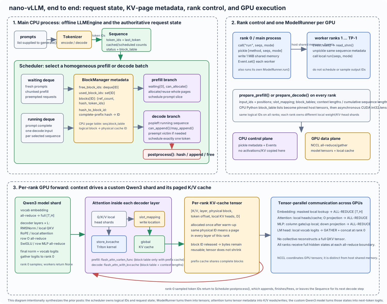
Read the diagram from top left to bottom right, but keep its three horizontal layers distinct:

1. The top-left panel is the authoritative CPU request state: Sequence objects, the waiting/running deques, and the BlockManager’s ID, reference-count, and prefix-hash metadata.
2. The top-right panel is rank control: rank 0 sends a small shared-memory command to worker ranks; every rank independently prepares local CUDA tensors from the same sequence metadata.
3. The lower panel is the GPU forward: model and KV-cache shards stay on their own rank; NCCL exchanges only the tensors needed by tensor-parallel math; rank 0 alone receives complete vocabulary logits and returns sampled IDs to the scheduler.

The arrows intentionally preserve details that are easy to erase in a high-level picture: a block_table contains physical IDs rather than K/V values; the BlockManager’s Python dictionaries do not live in the GPU cache; and NCCL collectives are separate from the Event/shared-memory control path.

There are three different kinds of state in the diagram. Keeping them separate prevents several common misunderstandings.

State	Owner and location	Examples	Lifetime
Request/control state	Main CPU process	Python Sequence, waiting/running deques, status, sampling parameters, block-ID metadata	One request or the engine run
GPU execution state	One copy per rank/GPU	model weight shard, graph buffers, per-rank KV-cache tensor, context tensors	ModelRunner lifetime
Cross-rank coordination	Host shared memory plus GPU collectives	pickle control payload + Events; NCCL all_reduce and gather	One command or one forward call

The shared-memory payload is not the KV cache or activation data. Rank 0 pickles the method name and small Python arguments, writes them into a fixed 1 MiB host-RAM region, and signals worker Events. Workers unpickle the same seqs metadata, then independently build their own small CUDA tensors. The large tensor-parallel communication happens later through NCCL inside the model. Part 2 and Part 3 cover those two mechanisms in detail.

2.1 Startup: build the engine before any request exists

LLMEngine.__init__() performs its construction in this order:

Config(model path, limits, TP size)
  → set global Sequence.block_size
  → spawn worker ModelRunner processes for ranks 1 … TP-1
  → construct rank-0 ModelRunner in the main process
  → load tokenizer and EOS ID
  → create Scheduler and BlockManager

Each ModelRunner then initializes the NCCL process group, selects its GPU, builds nano-vLLM’s Qwen3ForCausalLM, loads that rank’s local parameter shards, warms up, allocates a per-rank KV-cache pool, and—unless enforce_eager=True—captures decode CUDA graphs. The compact configuration exposes a few decisive limits:

max_num_batched_tokens = 16384
max_num_seqs = 512
max_model_len = 4096
gpu_memory_utilization = 0.9
tensor_parallel_size = 1
kvcache_block_size = 256

Those are defaults, not universal capabilities. The code also constrains tensor_parallel_size to 1..8, requires a block size divisible by 256, and clips max_model_len to the checkpoint’s positional limit. A production engine would make many more deployment, cache, parallelism, and model options explicit.

2.2 From generate() to finished text

The public API is offline batch generation. generate() first adds every supplied prompt, then repeatedly calls step() until both scheduler deques are empty:

for prompt, sp in zip(prompts, sampling_params):
    self.add_request(prompt, sp)

while not self.is_finished():
    output, num_tokens = self.step()

add_request() tokenizes a string (or accepts token IDs), constructs a fresh Sequence, and appends it to the scheduler. There is no socket accepting a request halfway through this loop. That is why Part 1 calls nano-vLLM an offline inference engine, even though its internals illustrate continuous-batching mechanics.

One step() is the critical hand-off:

seqs, is_prefill = self.scheduler.schedule()
token_ids = self.model_runner.call("run", seqs, is_prefill)
self.scheduler.postprocess(seqs, token_ids, is_prefill)

The mode is batch-wide: a step is a prefill batch or a decode batch, never a mix. The scheduler tries waiting prefill work first and returns as soon as it schedules any; only when it schedules no prefill does it select running decode sequences. As discussed in Part 1, an online wrapper with unbounded fresh arrivals would need an additional fairness policy to prevent decode starvation.

3. One step as a detailed data-flow trace

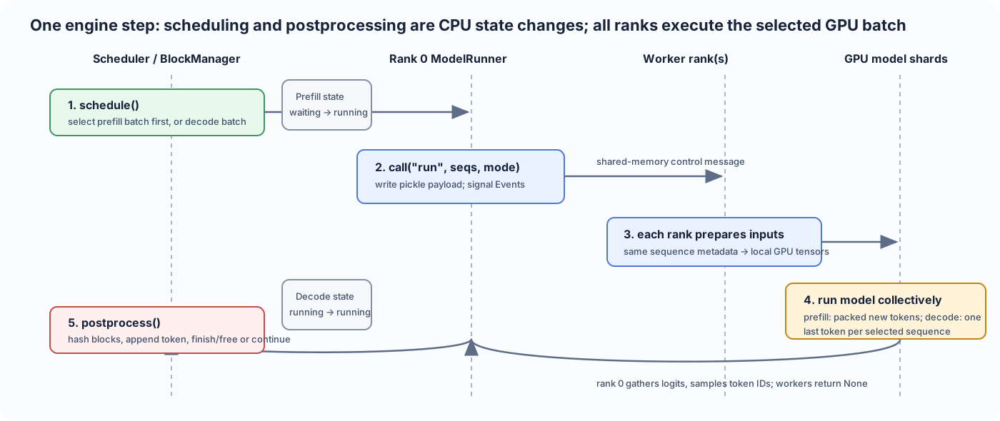
The diagram applies to both modes, with these important differences:

Aspect	Prefill	Decode
GPU input per selected sequence	not-yet-cached prompt slice	one already-sampled last_token
Batch tensor shape	packed total scheduled tokens T	one row per selected sequence B
Attention kernel	variable-length FlashAttention; optional prefix block table	flash_attn_with_kvcache over cached history
K/V work	write K/V for every new prompt token	write K/V for one input token per sequence
Output used by scheduler	first completion token only when prompt is complete	next completion token every step

The control/data divide is worth stating precisely:

1. The CPU scheduler reserves/reuses logical block IDs and returns seqs plus is_prefill.
2. Rank 0 writes ("run", seqs, is_prefill) to shared host memory, signals workers, and runs the same method locally.
3. Every rank prepares its own input_ids, positions, slot mappings, and block-table tensors on its GPU.
4. Every rank executes its Qwen3 weight/KV-cache shard. Tensor-parallel embedding and row-parallel projections all-reduce hidden states; vocabulary logits are gathered to rank 0.
5. Rank 0 samples the next IDs. postprocess() hashes newly complete pages, advances cached-token counts, appends output tokens when appropriate, and either frees finished K/V blocks or leaves the sequence running.

The main process is the authoritative owner of request objects. Worker processes receive deserialized copies for the forward pass; they do not decide scheduling order, mutate the central deques, or sample output tokens.

4. What performance numbers mean here

4.1 The repository’s published benchmark is useful—but narrow

The nano-vLLM README publishes one comparison on an RTX 4070 Laptop (8 GB) with Qwen3-0.6B: 256 requests; random input lengths 100–1024; random output lengths 100–1024; and a reported total output throughput of 1,434.13 tokens/s for nano-vLLM versus 1,361.84 tokens/s for vLLM. Repository README

The included bench.py explains the measurement better than a chart alone:

llm.generate(["Benchmark: "], SamplingParams())  # warm-up
t = time.time()
llm.generate(prompt_token_ids, sampling_params, use_tqdm=False)
t = time.time() - t
total_tokens = sum(sp.max_tokens for sp in sampling_params)
throughput = total_tokens / t

The benchmark uses ignore_eos=True, so every request produces its configured max_tokens; the numerator is consequently the total generated output-token count. It times one offline generate() wall-clock interval. It is a reasonable smoke test for this exact model, software stack, random-length workload, and laptop GPU. It is not a universal conclusion that nano-vLLM is faster than vLLM:

• it does not publish time-to-first-token (TTFT), time-per-output-token (TPOT), tail latency, queue time, cache hit rate, or peak memory;
• it does not measure continuous online arrivals, cancellation, streaming, multi-node execution, or models beyond Qwen3-0.6B;
• model version, vLLM version, CUDA/PyTorch/FlashAttention versions, power settings, and GPU clocks materially affect a comparison;
• the two systems deliberately offer different functionality, so equal total throughput alone is not equal serving capability.

This post does not manufacture replacement measurements: no compatible local CUDA testbed was used. The README values above are attributed repository results, not results from this blog.

4.2 A reproducible benchmark plan

A fair study should report a workload matrix, environment, metric definitions, and raw outputs—not a single headline throughput. The following matrix is a good minimum.

Experiment	Vary	Measure	What it isolates
Offline batch throughput	prompt/output lengths; number of sequences	prefill tok/s, decode tok/s, total tok/s, peak GPU memory	baseline engine behavior
CUDA Graph effect	enforce_eager=True/False; supported decode batch sizes	decode TPOT, CPU launch overhead	graph replay value
Prefix-cache effect	identical whole-block prefix vs no shared prefix	prefill time, cache hit blocks, KV usage	reuse versus recomputation
KV-pressure behavior	long concurrent sequences; constrained cache	preemption count, recomputed tokens, completion latency	scheduler/block-manager trade-off
Tensor parallelism	TP=1 versus each valid TP size	tok/s, scaling efficiency, NCCL time, per-GPU memory	compute/memory savings versus communication
Online serving comparison	fixed arrival rate/concurrency and a server wrapper	TTFT, TPOT, inter-token latency, p50/p95/p99, goodput	service-level behavior

For the last row, nano-vLLM needs an explicit wrapper before the experiment is meaningful: the repository itself has no HTTP server, no continuing admission loop, and no cancellation/streaming implementation. Do not call an offline 256-prompt batch a serving benchmark.

vLLM’s benchmark CLI distinguishes offline throughput, single-batch latency, startup, sweep, and online serving benchmarks. Its serving documentation reports client-observed total throughput alongside TTFT, TPOT, inter-token latency, and end-to-end latency, including selected percentiles. vLLM benchmark CLI vLLM serving benchmark

For any future results table, record at least:

model revision, tokenizer revision, dtype/quantization, GPU model/count,
GPU clocks/power mode, CUDA/PyTorch/FlashAttention/vLLM/nano-vLLM versions,
TP/PP/DP sizes, eager/graph choice, KV-cache settings, warm-ups, seed,
prompt/output distribution, arrival process, and exact metric formulas.

5. nano-vLLM versus vLLM V1

The current official vLLM architecture overview describes a multiprocess V1 system. An API server handles HTTP input processing and output streaming; an Engine Core owns scheduling, KV-cache management, and dispatch; GPU worker processes execute the model; and a data-parallel coordinator is added when data parallelism is used. API servers communicate with engine cores through ZMQ sockets. This is a substantial expansion of the small rank-0/worker arrangement in nano-vLLM.

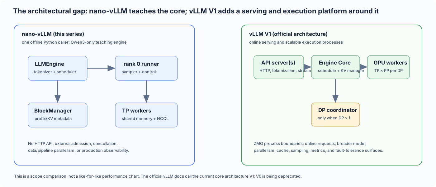
Concern	nano-vLLM	vLLM V1 direction
Primary interface	Offline LLM.generate()	Offline LLM plus online serving entrypoints and API-server processes
Scheduling	Compact prefill-first scheduler and two deques	Engine Core busy loop with production scheduling/cache management responsibilities
Process topology	Main rank-0 process plus TP workers, host shared memory/Event commands	API server(s), Engine Core process(es), one GPU worker per GPU, optional DP coordinator
Parallelism in this code	Tensor parallelism only; local ranks 1..8	Tensor, pipeline, and data-parallel process topology; feature availability depends on configuration/platform
Models	One custom Qwen3 implementation	Broad model/hardware support, with V1 support status varying by architecture and feature
KV behavior	Fixed per-rank GPU pool, block IDs, exact full-block prefix cache, recomputation preemption	V1 cache manager and richer execution surface; V1 explicitly reworked scheduler/cache/worker/sampler/API core systems
Request lifecycle	No server admission, cancellation, deadlines, streaming, or external load balancing	API input processing, streaming, routing across engine cores, metrics, and production-oriented coordination
Sampling/features	Temperature-only categorical sampling	Broader but evolving serving/model feature surface; check V1 status per feature
Observability/benchmarking	tqdm prefill/decode rates and one simple script	benchmark suite, service metrics and process-level operational surface

This table should not be read as “vLLM is merely nano-vLLM plus an HTTP server.” vLLM’s V1 architecture expands the inference core into a process architecture with an API server, Engine Core, GPU workers, and optional data-parallel coordination. Feature support and operational behavior are version-sensitive, so a production deployment should check the current documentation rather than infer support from a broad comparison. vLLM architecture overview

5.1 The real lesson of the comparison

nano-vLLM exposes the irreducible inference mechanics:

admit a sequence → allocate/reuse KV pages → choose prefill/decode work
→ run a model shard → store/read K/V → sample a token → update state

vLLM V1 must make those mechanics reliable and efficient under continuing traffic, more model families, richer output policies, heterogeneous hardware, multiple parallelism dimensions, and operational failure modes. The additional architecture is not accidental complexity; it is the cost of those requirements.

6. Series conclusion

The useful mental model for this entire series is a chain of stable interfaces:

prompt text
  → token IDs in a Sequence
  → scheduler decision and logical block IDs
  → per-rank GPU tensors, block tables, and KV slots
  → custom Qwen3 layer shards and NCCL collectives
  → rank-0 logits and sampled token ID
  → postprocess: append, free, preempt, or run again

Once that chain is clear, the larger vLLM architecture is less mysterious. Its API servers, Engine Cores, workers, cache managers, parallelism controls, and benchmarking tools are extensions around the same core contract—designed for workloads that nano-vLLM intentionally leaves outside its small, readable offline engine.